Category: My Dataviz

UEFA inequality

Long winding Intro

One of my least controversial opinions is that soccer is incredibly boring to watch, and that people who are passionate supporters of a club (or national team) tend to be incredibly annoying. That makes me an expert on the subject. And this being a FIFA World Cup™ (® 2026 Jared Kushner and co.) year and all, I figured I could make a plot or two about the Beautiful Game. It was actually the UEFA Champions League that inspired me for this post, but I couldn’t quite meet my target of finishing the article before this year’s champions league finals.

What caught my attention is that England seems to have quite a few teams that are doing well at the continental-level contests. Additionally, the (English) Premier League has a “Big Six” of top-tier teams, which should provide for a high-quality competitive national league (please ignore the fact that one of those teams has been on the verge of relegation for the past two years). Meanwhile, the national leagues of other European countries seem to be dominated by two or three clubs that are much richer and powerful than others. Because of this, they are derogatorily called “Farmers Leagues“.

But even looking just at the Premier League, I get the impression that things are much less competitive than what I remember from the national league in Brazil back when I was growing up in the 90s. Manchester City’s record-breaking 2017–18 season had them winning the championship with 34 wins, 4 draws, and just 2 losses, totaling 100 points. The following two seasons were won by Manchester City again with 98 points, then Liverpool with 99 points.

So here’s my idea: what if I used the Gini index to quantify this hoarding of points in a league by the top teams? Would that be a good indicator of inequality of performance, or the “farmness” of a league? And if so, could it reveal which national leagues are more competitive than others?

When I graduated I took a small oath that said I should be clear and honest in reporting my scientific results, such that society can rely on my judgement. So take this as a disclaimer to not take any of this article seriously. However, just to add a little faux-rigor to the proceedings, I am laying out some hypotheses before I get the results:

Hypothesis #1: the Gini index is adequate in setting apart a more “one-sided” league from a more “evenly-competitive” one.
Hypothesis #2: the Premier League has less inequality than the other top-level domestic leagues in the “Big Five” (Spain, Germany, Italy, and France).
Hypothesis #3: the Brasileirão (Brazil’s top league) has less inequality than the top-level domestic leagues in the Big Five.
Hypothesis #4: inequality in championship points is correlated with inequality in wealth between teams.
Hypothesis #5: I can come up with a different metric that is a better indicator of a league’s farmness than the Gini index.

Sourcing the data

Very little data is needed for this exercise, only the overall championship table with the points earned by each team. Maybe it’s just me not being a sports guy, but Wikipedia is where I would go to look for this type of information. Thanks to whatever saint made a “League Table” template, the format is almost identical in the (English language) Wikipedia page of every national soccer championship.

Since it looks so easy, I figured I should download the results from every top-level league in the European soccer confederation. I don’t know where they get all these countries, but there’s apparently 55 UEFA members. All but Liechtenstein have their own domestic league. I mean, even the Faroe Islands have a complete system including a fourth tier league.

To get more robust conclusions and to capture changes in inequality over time, I wanted to get the last 12 years or so of seasons (three 4-year World Cup cycles). I don’t remember why, but I ended up extending that to results going back to 2013. For the championships scheduled over a calendar year, the range was from 2013 to 2025. For the championships that follow a (Northern-hemisphere-centric) school year format, the range was from 2012–13 to 2025–26.

To compare against these unequal Europeans, I also got the data for the leagues in Brazil and the United States, since I previously discovered that I am 43% American. After all, these are the two countries with the most World Cup titles (see here and here for more information; and no, West Germany is not a real thing). The combination of the aforementioned Big Five with Brazil and the US is henceforth referred to as The Seven, as that is the focus of the analysis. I later grabbed more data for The Seven going back to the year 2000.

After writing some scripts, sieving out the results with Beaultiful Soup, and manually fixing countless edge cases, I ended up with 858 seasons worth of data, totaling 12,210 rows. It’s never “too easy”…

Inequality in points earned is compared in the analysis against a few other variables, so there are some extra sources of data needed. “UEFA Association club coefficients” are taken from UEFA. Country income inequality is taken from the World Bank. And club and league market values are taken from Transfermarkt.

Game Gini

Introduction 2

The Gini coefficient, which I am calling index to be more space-efficient, is an indicator that quantifies income inequality. But although measuring income inequality (and sometimes wealth) was its original purpose, I don’t think anyone can stop me from applying it to some other variable, such as points in a competition. The Gini index is basically the ratio between the integral of the line of cumulative sum of income from the lowest to highest earner (or our alternative variable of interest) and the integral of the same cumulative curve but if income was equally distributed.

For our discrete case, I applied the following formula to each season of each league:

G = \frac{\sum_{i}^{n}{\sum_{j}^{n}{\abs{x_i-x_j}}}}{2n^2\bar{x}}

where $x_i$ is the amount of points team $i$ (out of $n$ teams) won in the championship. I only considered results in which the team was listed as having more than zero games played and at least zero points. Why do I even have to say that? Let’s explore the dataset a bit before the main results…

Stand-out performances

There were 39 instances of a team finishing the season without a loss, but only one case in which a team won every single game (i.e. no draws). The Lincoln Red Imps won all 10 games of the 2021–22 Gibraltar National League. However, although I only considered the first phase of the tournament with all 11 clubs, the top 6 then participated in a playoff called the “Championship Group”, and the Red Imps only won 9 of those 10 extra games, with Europa FC achieving a heroic 3-3 win against them. The wiki page of the Red Imps also says they hold the European record of 88 straight unbeaten games, achieved between 2009 and 2014. This GOAT team also has the highest season goal difference in my dataset: 121 GD (130 goals for, 9 against) in the 27-game 2015–16 season.

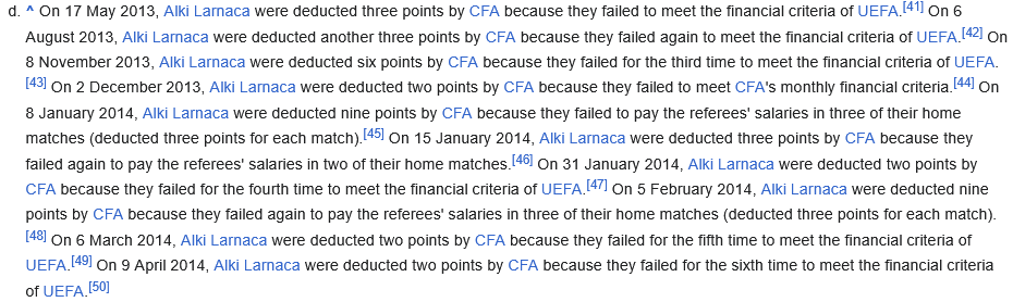
On the other hand, FC Florești finished the 2021–22 Moldovan National Division with zero wins, zero draws, 28 loses, and negative 6 points. They were excluded from competition after 19 games for match-fixing allegations, with their remaining 9 matches ordered to be considered “administrative loses”, and they received a 6-point deduction for this alleged match-fixing. But that’s peanuts. The lowest amount of points in the dataset was −29, achieved by Alki Larnaca in the 2013–14 Cypriot First Division after a 0-2-24 record:

Here are the actual results

After crunching all the numbers, here is what I found:

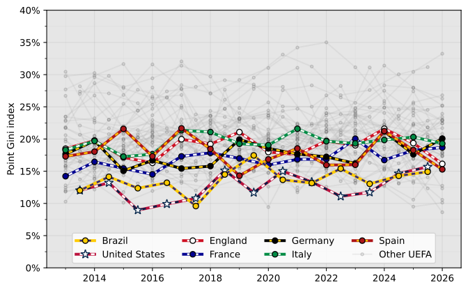
It was hard to find a suitable style for this plot. To achieve seven distinct enough lines, I resorted to multi-colored dashes and markers. The U.S. line is even fancier with three different colors and a star as the marker, honoring its starry flag. All of this really adds to the clutter, which is why I’m not really happy with how this, the main figure of the article, looks. I also had to go with a gray background, which I tend to avoid, in order for the white markers to stand out a bit more. I am unsure if the “Other UEFA” lines are too faint or not, I guess it depends on how well your monitor displays gray colors.

As for the results, they do support hypotheses #1 (the Gini index can indicate, to some extent, inequality in point distribution) and #3 (Brazil’s league is more equal than those of the Big Five). Except for one point, the Gini of Brazil and the U.S. are all below the lines of the Big Five. But the results don’t really support hypothesis #2: England has a similar point Gini to the other four European countries in focus.

I was also curious if there were any significant trends over time, but there was nothing really obvious in the plot. So I went back and grabbed more data, just for The Seven, going back to the 1999–00 season. The Brazilian data series starts from 2001 because the 2000 tournament had a different, weird, format. I also changed the presentation a bit to focus on the comparison between the Gini of Brazil and the others:

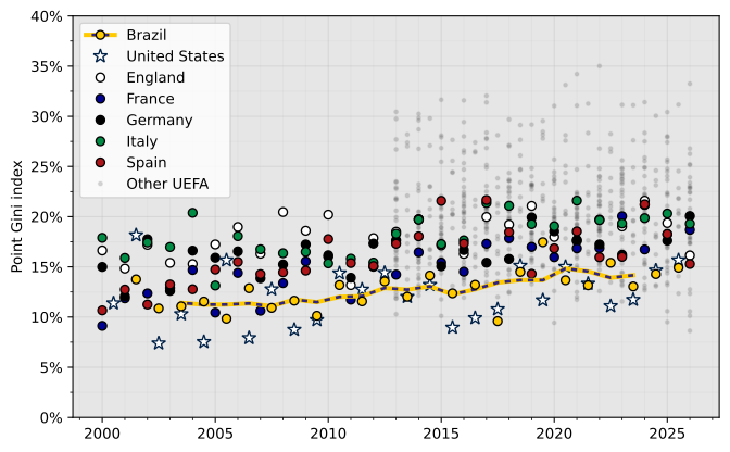
So I guess inequality crept up over time, as I would have guessed, although maybe not by much. At least according to the Gini index.

Going back to the 2013-onwads dataset, I checked to make sure that the metric was robust with regards to the number of teams on a league:

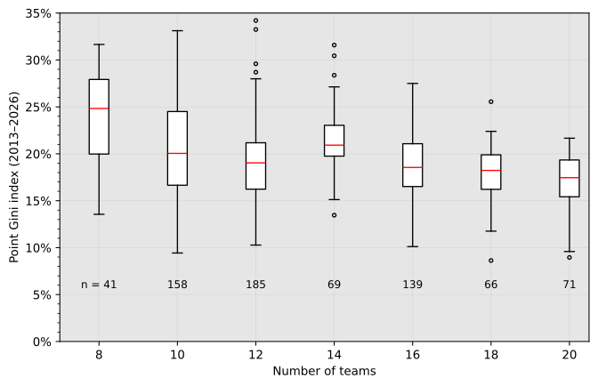
That seems to me quite solid. Perhaps the 8-team leagues are a bit more unequal, but, as those notes from the Gibraltar league exemplify, the really small leagues can be quite ~~weird~~ exceptional.

Here’s a full picture with the 56 countries ordered by the median “seasonal” Gini:

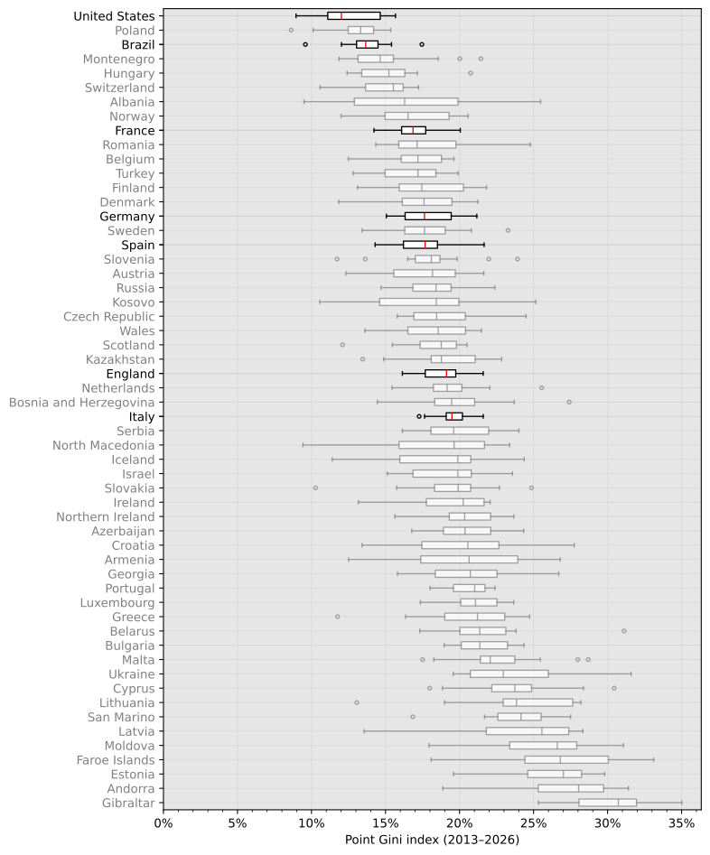
This is a better way to visualize that, indeed, Brazil and the U.S. have lower Ginis than almost any European country.

Now let’s recall the original inspiration for this article: the UEFA Champions League. Every year the best clubs at each European domestic league are invited to play in it, and the number of spots each country gets depends on the past performance of their clubs at continental competitions. Specifically, the UEFA coefficient is calculated using a score based on the past five seasons of European competitions. Comparing the UEFA coefficient to the point Gini index should tell us if there is some correlation between the strength of (the top performers of) a league and its point inequality:

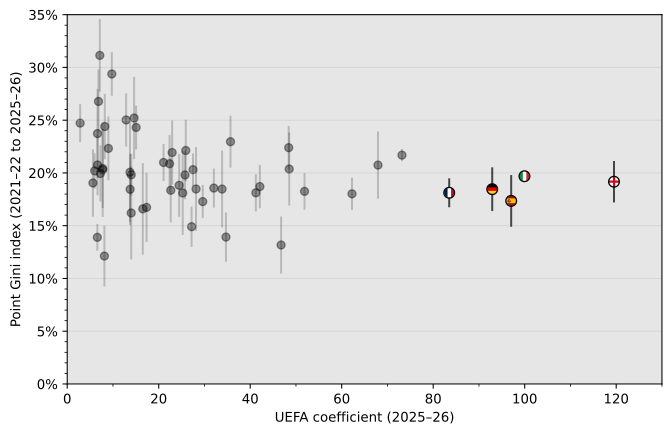
UEFA coefficients actually fluctuate more than the point Gini index over a period like 5 years, but I opted to keep only the vertical error bars above to keep the focus on the Gini index. The UEFA coefficient is just a proxy here for how high the performance level is relative to other leagues. And it doesn’t really look like there is a correlation between the variables. I.e. leagues that do better at European competitions are not necessarily more (or less) “competitive” themselves.

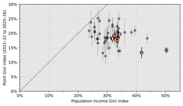
Just for fun, I thought it would be nice to compare our point Gini to the o.g. income Gini of each country. I didn’t expect a correlation, but at least this plot shows the difference in magnitude between the two. The closest we get to equality of inequality between soccer and population income is ~~soviet(?)~~ Belarus: 23.7% vs. 24.4%. Also, we can see Brazil and the U.S. are not just powerhouses in soccer; income inequality is a proud national tradition (Turkey is the second highest in the dataset, by the way).

Market value

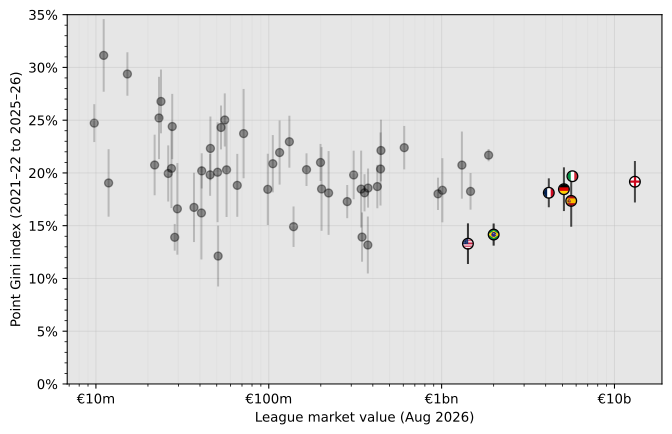
Another way of ranking leagues is by the total market value of its players. I have no idea how Transfermarkt arrives at their numbers, but I am taking them at face (euro) value. From the plot, it also doesn’t look like there is a big correlation between point Gini and the market value of a league. Note that I did not normalize value by number of teams or number of players per team.

The more interesting question though is whether inequality in team market value is associated with inequality in points earned. To investigate, I obtained from Transfermarkt the market value of each team for each season of The Seven leagues. The data available goes as far back as the 2004–05 season for the Big Five, and the 2006 season for Brazil and the U.S. However, especially for the latter two, there are a lot of players with no listed value in the early seasons, which I treated as zero value. Because of this, I split the data roughly in half: pre-2015 and post-2015 (which includes 2015). But before getting into inequality, let me just plot points earned versus team value:

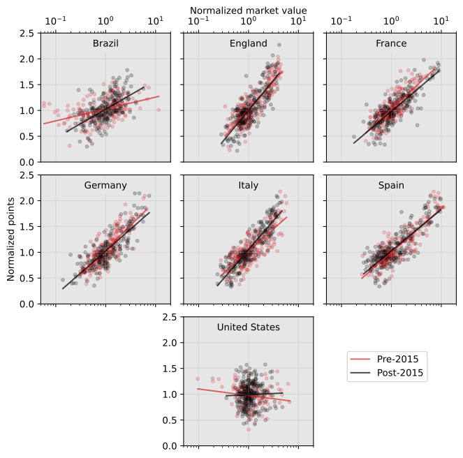
I think this is the nicest plot out of the dozen or so I made for this article. Unfortunately, it’s not really directly about inequality, otherwise I would have put this as the featured image. It clearly shows why players that earn more money earn more money: they win more points.

Well, except for the U.S. I genuinely don’t know how to explain this. My best guess is that in the Major League Soccer everything is made up and the points don’t matter? I mean, the team that wins the most points is not necessarily the champion: the top teams (currently 18 out of 30!) go to a playoff to determine that.

But still, I was hopeful there would be some correlation between the Gini index of points and the Gini index of team value. This is the result:

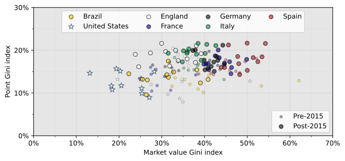
The pre-2015 are a bit all over the place, so let’s disregard them. And add some linear regression lines for good measure:

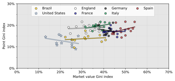
So maybe there is a faint pattern across different leagues, in line with our hypothesis #4. There is a trend of increasing both Ginis if we go from the centroids of U.S. -> Brazil -> Germany -> Spain. But there isn’t really a significant correlation of Ginis within each league.

I would speculate, using my credentials of soccer expert who doesn’t follow or like the game, that the Gini index of points fluctuate too much within consecutive seasons due to the random nature of such sport; look back at the time series plot. And likewise the Gini index of market value is too sensitive to a few big transfers, which might or might not pay off immediately. Because of that, it’s hard to get a good signal of a correlation, especially within just twelve or eleven seasons. The underlying inequality within leagues is more structural, not something that has easily observable changes from year to year.

Anyways, all these analyses were fun, but I didn’t feel like the Gini index really captured the particular sense of inequality that I got from these European leagues. Therefore, in the last part of this article, I try to come up with a different metric to evaluate how “competitive” each league is.

A metric candidate

Motivation

What I think is the key factor in whether people perceive a league as competitive or as a farmers league is the amount of teams that are in contention for the title. If a single team dominates and runs away with the title with a large number of rounds left to go, the league will be seen as not-competitive, regardless of how well distributed points are amongst all other teams. Conversely, if multiple teams fight for the title until the end, everyone will be excited about that and no one will care about how low on points the teams at the bottom of the table are.

Therefore, I wanted a metric that condensed to a single number the size of the field of teams that are credibly in contention for first place. My idea was to determine a point threshold (with uncertainty) above which a team is considered a potential candidate for the title. The amount of points (with uncertainty) that could be expected from each team would also de determined. The likelihood of each team reaching the “candidate zone” would be summed together and the result is the Candidate coefficient. I think I’m using “coefficient” here instead of “index” because it feels wrong to call it an index when it’s not a number in the zero to one range. The Candidate coefficient is thus a sort of indicator of how many different candidates (to be champion) there might be in a league.

But what should the threshold be? The obvious alternative would be the amount of points achieved by the team in first place, but that’s too rigid. Maybe 3 points lower than that? 6 points? Eventually, I found a good solution that is not completely arbitrary. The plot below shows the histogram of how much a team’s total points earned changed from one season to the next:

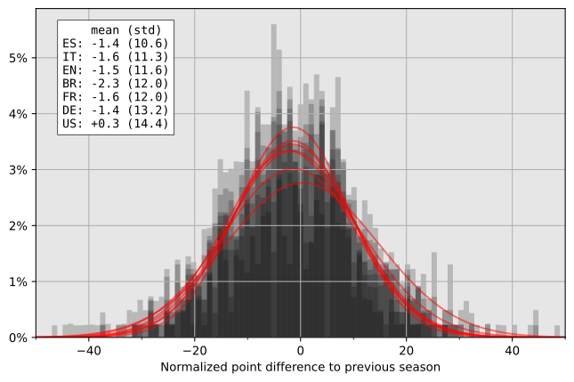
It is interesting to see that the mean change is not quite zero. That could be explained by the relegation system. Teams that oscillate every year between first-tier and second-tier leagues are not going to be represented in the histogram. Teams that are usually in the top league but eventually end up relegated have their bad season captured in the data, but not their bounce-back season when they return. This bias would explain the negative averages. Since the Brazilian league relegates 4 teams every year instead of 3 like in the European leagues, that effect is larger. The U.S. does not have a relegation system, so the +0.3 average is probably just due to a slight increase in average points per game over the seasons.

Definition

But the reason why I made that plot is that I could use its data as a metric of “how much can we expect a team’s score to change from one season to another”. I defined that the threshold ( $T$ ) to be considered a “candidate” is the average points of the best team in the league (other than the team you are calculating this for) minus the standard deviation of the point difference between seasons, considering every team in the league and all the seasons in my dataset (between 1999–00 and 2025–26). I.e. I used a constant value ( $D$ ) specific to each league, in order to somehow incorporate the fact that, for example, teams in the American league have more year-to-year variation in results than in the Spanish league. The rationale for this threshold parameter is that if your team finished that close to the winner, you can at least have a reasonable hope that maybe next year will be their year, so it’s okay to consider them a “candidate”.

For each team ( $i$ ) playing in a season ( $y$ ) of a league, a “points expected” variable ( $X_{i,y}$ ) is determined. The points expected from a team are defined as a random variable having a normal distribution with the same average and standard deviation as the amount of points per season for that team in the last 5 seasons. I could have used rolling windows centered at the season to which the Candidate coefficient is being assigned, but I wanted something more comparable to the Gini index; using thus the season for which the calculation is being made and the four preceding seasons. For teams that did not play in all of those five seasons, only the seasons with them are taken into account in their part of the calculation. If a team has not played in any of the four preceding seasons or if the standard deviation is lower than 3 points, the standard deviation of the “points expected” distribution is set at 3 points—this is unlikely to make a big difference because these should be mainly teams close to the bottom of the table.

The Candidate coefficient ( $C_y$ ) for a league at year $y$ is the sum for all teams of the probability that the points expected ( $X_{i,y}$ ) is larger than the threshold( $T_{i,y}$ ). I didn’t mention it until now to not complicate the explanation further, but all calculations are made using points normalized by the numbers of games in a season ( $x$ ), to account for different numbers of teams in different leagues and years. Note however that the Candidate coefficient is not itself normalized, so larger leagues could have higher numbers, so long as those extra teams are also fighting for the title. Here’s everything put together:

\begin{array}{rcl} D & = & \mathrm{std}\left(x_{i, y}-x_{i,y-1}\right)_{i=1, …, N;\ y=2000–01, …, 2025–26} \\ X_{i,y} & = & \mathrm{N}\left( \mu{}=\mathrm{avg}(x_i)_{y-4, …, y},\ \sigma{}=\mathrm{std}(x_i)_{y-4, …, y} \right) \\ T_{i,y} & = & \mathrm{N}\left( \begin{array}{rcl} \mu{} & = & \mathrm{avg}\left(\max\left(x_j\right)_{j\ne{}i}\right)_{y-4, …, y}-D \\ \sigma{} & = & \max\left(3.0,\ \mathrm{std}\left(\max\left(x_j\right)_{j\ne{}i}\right)_{y-4, …, y} \right) \end{array}\right) \\ C_y & = & \sum\limits_{i}{\mathrm{P}\left(X_{i,y} > T_{i,y}\right)} \end{array}

Results

Plotting the Candidate coefficient over time gives a similar picture to the Gini index:

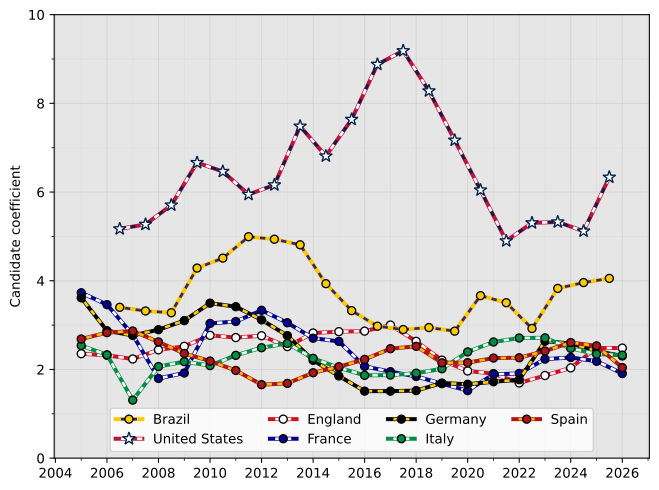
The Brazilian league is again “more competitive” than the Big Five (hypothesis #3 ✓) . The English are not much less farmers than the rest of the Big Five (hypothesis #2 ✗). The main difference here seems to be that the MLS is in a league of their own (I guess they all are in a literal sense).

Peeking under the hood, this is what each score is made of for the latest season:

🇺🇸 6.3	🇧🇷 4.1	🏴󠁧󠁢󠁥󠁮󠁧󠁿 2.5	🇮🇹 2.3	🇩🇪 2.3	🇪🇸 2.1	🇫🇷 1.9
San Diego FC .91	Palmeiras .84 🏆🏆	Manchester City .82 🏆🏆🏆	Inter Milan .90 🏆🏆	Bayern Munich .91 🏆🏆🏆🏆	Real Madrid .86 🏆🏆	PSG 1 🏆🏆🏆🏆🏆
Los Angeles FC .53 🏆	Flamengo .67 🏆	Arsenal .68 🏆	Napoli .57 🏆🏆	B. Leverkusen .50 🏆	Barcelona .85 🏆🏆🏆	Lens .29
Phil. Union .47 🏆	Mirassol .52	Liverpool .56 🏆	Milan .37 🏆	B. Dortmund .37	Atlético Madrid .14	Marseille .19
FC Cincinnati .44 🏆	Botafogo .48 🏆	Man. United .12	Como .15	RB Leipzig .19	Girona .09	Monaco .13
Inter Miami .43 🏆	Atlético Mineiro .42 🏆	Chelsea .10	Juventus .08	VfB Stuttgart .15	Villarreal .03	Nice .10
Columbus Crew .37	Internacional .23	Tott. Hotspur .08	Atalanta .07	Union Berlin .06	Athletic Bilbao .03	Rennes .08

Candidate coefficient for the 2025 or 2025–26 season, with the six highest team contributions per league listed. The number of times a team placed first in the last 5 seasons is indicated by 🏆 symbols. U.S. results concern only the regular season.

The U.S., and to a lesser extent Brazil, has so many teams that are hovering close enough to the “target” zone. Note that the specific teams that show up at the top change significantly over the years, even if the total Candidate coefficient doesn’t, with teams that have won a championship in the five-year analysis window dominating the statistic. For the 2025 U.S. coefficient detailed in the table above, San Diego FC is a bit of an anomaly because 2025 was the team’s first ever season, which they finished three points away from first place. Meanwhile, Paris Saint-Germain won all 5 of the latest Ligue 1 seasons, which is why their coefficient is 0.9998.

These results made me wonder: perhaps this entire article and all the work that was put into it could have been replaced by just looking at how many different winners each league had in the last number of years. This is orders of magnitude simpler and gives a more direct idea of how much diversity a league has at its top.

Number of different champions in the last 20 seasons {times won per team}:
- United States: $13: \{3, 2, 2, 2, 2, 2, 1, 1, 1, 1, 1, 1, 1\}$
- Brazil: $8: \{4, 4, 3, 3, 2, 2, 1, 1\}$
- France: $8: \{11, 2, 2, 1, 1, 1, 1, 1\}$
- England: $6: \{8, 5, 3, 2, 1, 1\}$
- Italy: $5: \{9, 4, 3, 2, 2\}$
- Germany: $5: \{15, 2, 1, 1, 1\}$
- Spain: $3: \{11, 7, 2\}$

Looking at the list above, it’s hard to argue against the farmers league allegations concerning the Bundesliga and La Liga. Bayern Munich won 15 of the last 20 seasons, while Real Madrid and Barcelona won 18 of 20. Ligue 1 has a diverse list of champions, but PSG won 11 out of 20 while no other team won more than twice in the same period. It could be worse though: the last time a team other than Celtic and Rangers were Scottish champions was 1985.

Meanwhile, the U.S. is just built different. 13 different champions in the last 20 seasons. I get the same number whether I look at regular season or playoff, by the way. And this is perfectly in line with the other Big Four major leagues (lots of “Big [number]” in sports apparently): NBA (12), MLB (12), NFL (13), NHL (13). I don’t know how they achieve that in the MLS without a draft system, but it really seems like anything can happen in the land of opportunity.

Also, I am now ~4500 words, 12 figures, 3 lists, 2 sets of equations, and 1 table deep into this article, and only now that I looked at the list of MLS champions have I realized that the league also includes Canada. I will ignore this revelation, keep the American flags and keep the “U.S.” or “United States” shorthand for the league. I could link to a Truth about the imminent (re?)unification of the two countries, but I already did that in the last post.

Taking a step back to the original plan of Gini index and my Candidate coefficient, here’s a comparison between them:

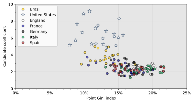
Largely correlated, if I can be charitable to myself here. At least the Candidate coefficient better captures how distinct the U.S. league is compared to the Gini index.

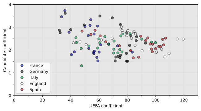
There is still no sign of a correlation between our inequality metric and the UEFA coefficient:

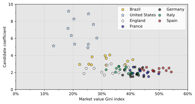
And finally, there is something in terms of market value inequality being correlated with performance inequality. But like the Gini index, the Candidate coefficient only shows a significant difference between leagues, not between seasons within them:

Having said all of that, I am not sure if I can say the new metric I came up with is better than the Gini index in representing the “farmness” of a league (hypothesis #5). But at least exploring this idea led me to some interesting realizations.

Conclusions

Analyzing sports data is much more interesting than watching sports. Well, at least for soccer.

Oh, and I can make plots with a gray background that I don’t look straight from Windows 95. It still reminds me a bit of Windows 98 though.

August 23, 2026

Country codes

Long winding intro

Imagine someone has a computer model of the Earth and its atmosphere. The atmosphere may be represented by a 3-d grid. If we ignore the vertical coordinate, you may have a regular latitude × longitude grid.

Let’s then say you use a related computer model to investigate the effects some emissions have on the atmosphere. And then use those results to estimate the associated impacts this pollution has on human health. You would do so using epidemiological data, which are heavily dependent on healthcare and socioeconomic conditions (among many other factors), and that are produced and compiled at national levels. Can you imagine such a study?

What you would have, in this theoretical scenario, is a need to figure out what country each of your politically ignorant grid cells is in. It seems trivial, but the thing about political borders is that there is always some trouble with edge cases.

In this post I will go over some interesting things I found along the way of making such an assignment of countries to grid cells. There is no “one nice plot”, but rather a collection of small maps that will guide us on a world tour of a selection of country borders.

Where am I?

More precisely, how do you find out the name of a place given its geographical coordinates? Well, there is a fancy name for that: reverse geocoding. To give an analogy that is understood by only a vanishingly small number of people: it’s like looking up a number on the phonebook instead of looking up a name.

I had a regular grid of the globe with a cell every 0.5° in latitude and 0.625° in longitude. At a latitude of around 36° this is equivalent to 56 km by 56 km, if I did the math right. My solution was to reverse geocode the coordinates of the center of each of the $361\times{}576\approx{}208\ \mathrm{k}$ cells (the polar cells are half-sized in latitude, hence the 361). To be honest, I actually ignored the North Pole and everything south of New Zealand, but you get the point. I did so using OpenStreetMap through the Nominatim API. For each grid cell, I saved the two-letter code of the country in the address returned by the API.

Yes, country borders don’t quite align with the grid, but I thought that would be good enough. And it kind of was, except for two problems…

The first issue is that a very large number of cells are in remote areas of countries where the reverse geocoding doesn’t return anything. Regions like Siberia, the Amazon, the Sahara, the Outback, and the Arctic Archipelago.

The second issue is that in coastal regions, where a lot of people live, there is around 50% chance that the grid cell center will lay on the water. Sometimes Nominatim would give an (inland) address anyways, but more often than not it wouldn’t give a result.

In hindsight, I should have instead used a dataset of country boundary lines, which should solve the first issue, almost all of the second issue, and be more agnostic to resolution (208 thousand lookups is quite of a lot). I would then check the area of the intersection between each cell and the country borders, or at least check whether the cell is inside a border. However, even with this solution I would still have to deal with the issue of cells containing a border between countries.

Back to what I actually did, my goal was to assign a country to every populated grid cell. You can’t have human health impacts if there are no humans (taps side of head); environmentalists love this one simple trick. So I could just ignore the oceans and other big bodies of water. But because I thought of maybe using these data for other purposes (such as categorizing aircraft emissions by their location), I wanted to fill in the interior unpopulated gaps within countries.

To do this task, I exported the country code data to a CSV file and opened it in Excel. Zooming out revealed a perfectly projected plate carrée world map. This made it easy to manually bucket-fill the large inland gaps.

I use MS Excel® for all my GIS needs. North Africa seems to be peeling off, which is not good.

Resolving the issue of missing data for all populated grid cells, however, would prove to be a bit more laborious. The biggest problem is when one of those lies along the border of multiple countries. My simplistic methodology assigns a single country to each cell, which means I would have to make some choices in those cases.

Population counts

Because of reasons, I was using the LandScan 2019 global population dataset. It contains the population count on a much finer resolution of ~1 km, which I then aggregated into my coarser grid.

It would be easier to assign each grid cell to the country with the most area inside of it. But the more correct approach here would be to give the cell to the country with the largest population within it.

A first plot

This is where today’s plots come in. I wanted to quickly check some edge cases, figure out why the reverse geocoding didn’t return anything, or decide what makes the most sense when a cell lies on the borders between multiple countries.

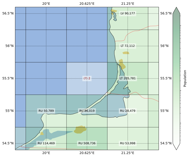
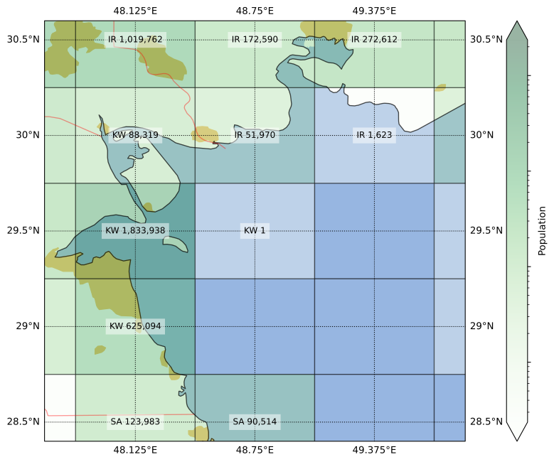
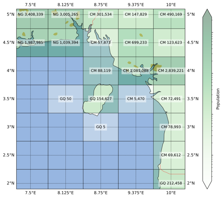
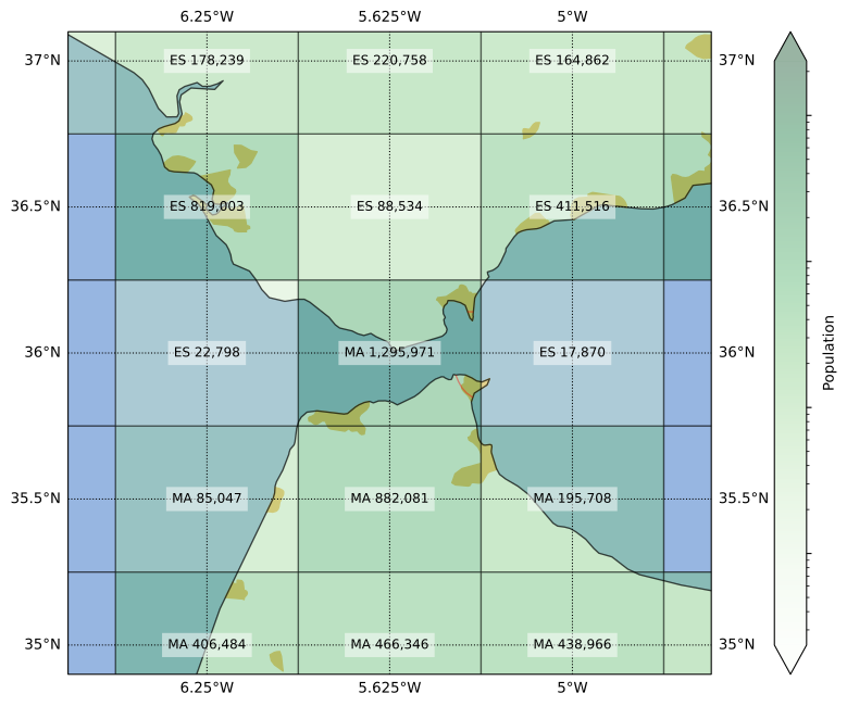
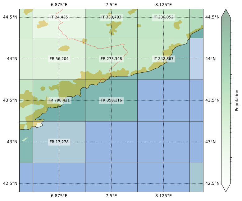
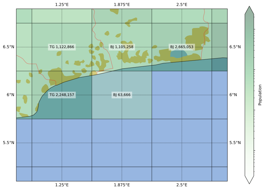
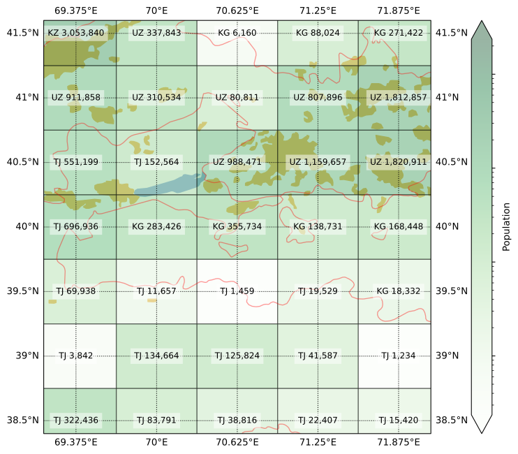
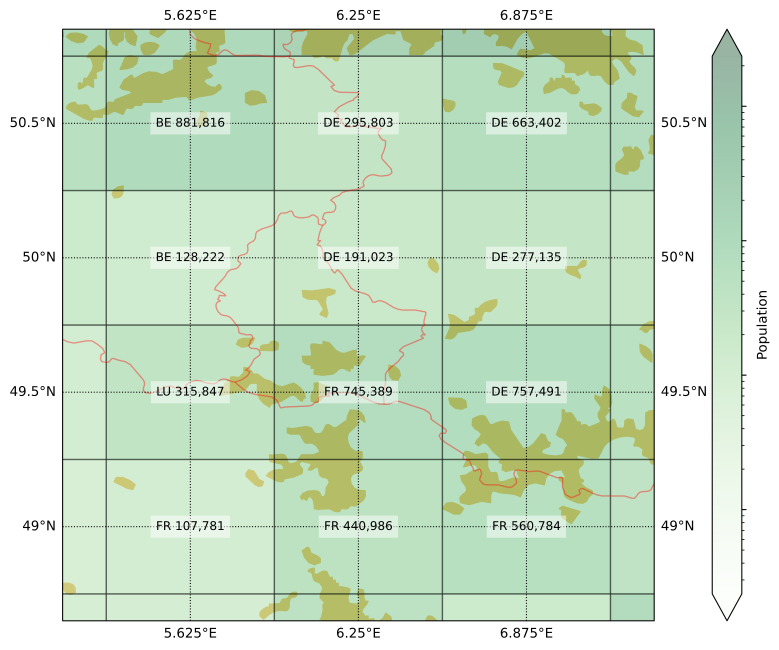
I made short function using Cartopy that takes the coordinates of the center and some lat/lon margins. The output is a little map with several features: coastlines, country borders, large water bodies, and urbanized areas. The population count for each grid cell and the already assigned country code are printed in front of a semi-transparent white box. Each cell is also (semi-transparently) shaded based on its population.

Here is the first example, ~~Königsberg~~ Калининград:

For this figure I left the “problem cell” with no country code, to give an idea of what the assigning process looked like. The remaining plots already show the country codes that were ultimately assigned.

You can see in this first plot that the grid cell center was in the water, but the cell also contains land from two countries. Lithuania was only ever so slightly clipped, so I assigned the cell to Russia. The impact of this was completely insignificant however, as the total population count here was 2 (two).

Going on a world tour

But of course, we I can always do even less useful work. To start off our world tour, the Persian Gulf:

The image actually undersells the situation, as the population counts are rounded up to the nearest integer. The grid cell edges of the native resolution Landscan dataset don’t perfectly align with those on the target grid I’m using, such that sometimes the population in the finer cell is split half-and-half between two coarser grid cells. In the case of the cell at the center of the figure above, the aggregated population totaled ½ person.

Although this area looks completely on water, further inspection shows that it contains some islands too small to show up in the coastlines dataset. From what I can tell, this half-person populates the island of Auhah (Ouha? عوهة؟), owned by Kuwait. Youtube provides a couple of views of what’s like in this far-away^* piece of land (^*depending on where you are when reading this).

The Landscan population data is produced in part by processing satellite pictures. Despite having no permanent residents (I guess), this small island has a few small shacks, and a convenient heliport. Hence, this is what the pop data looks like:

I’m setting up a tracker to wait for something here to become available on Funda. Source: LandScan 2019.

But sometimes, the island in question has hundreds of thousands more people than that. And it doesn’t always belong to the country with the nearest shores. Our second stop, the island of Bioko, illustrates this:

Despite being much closer to Cameroon, Bioko is part of Equatorial Guinea. In fact, until a few months ago, that’s where country’s capital was located, in the city of Malabo. It’s a unique place with a quite interesting history, one that my South-American-educated self was unaware of before this tour.

For example, Equatorial Guinea has the distinction of being the only African country where Spanish is an official language (if you ignore Western Sahara). Although some people in Bioko speak an English-based creole called Pichinglis, due to the complicated history of, hmm, intercontinental migration around the 18th and 19th centuries.

Speaking of intercontinental, our third stop is the strait of Gibraltar:

About half the central grid cell above is on water, but the two bits of land across the strait have a peculiar setup. On one side there is the only part of the UK in continental Europe; which, I just learned, voted 96%-to-4% to remain in the EU. On the other side is a part of the transport infrastructure supporting key elements of the supply chain of the Dutch pharmacological industry. I mean, it’s one of the bits of Spain in Africa.

What made me double-check this cell was that it was originally assigned to Spain (nobody expected it). If you recognize that yellow blob of urbanized area in the southwestern corner as Tangier, that assignment might sound wrong. Indeed, although most of the cell’s area is in Spain, most of the population is in Morocco, so I made the adjustment. The territory of Gibraltar itself, with a population not much larger than 30 k, does not have its “GI” country code show up in the gridded dataset.

All else being equal, I would have given preference to a country code that doesn’t appear elsewhere, as the extra diversity might increase the robustness of the overall calculations (i.e. outliers would at least have some impact on the results). But sometimes, a single grid cell is the only place where multiple country codes occur. Fourth stop, the Leeward Islands:

More specifically, the island of Saint Martin. This is where 100% of the border between France and the Netherlands lies—until they put up a wall between Wallonia and Flanders, that is.

Although a bit smaller, the more funnily-spelled Sint Maarten has more people than the Frenchly-pronounced Saint Martin, which is therefore not represented in the final dataset. It is interesting that five neighboring cells in this region have five different country codes, a sign that our grid struggles to resolve the complexity of the Caribbean political landscape.

But the French get their revenge elsewhere. Fifth stop, la Côte d’Azur:

Monaco is almost entirely in this one grid cell whose main ingredient is Mediterranean water. Still, most of its land area is in France. Even though the center of Nice falls outside of this cell, the total population of Monaco is only around a tenth of the cell’s pop count. Because of that, I could rest easy that the “MC” omission was correct.

Speaking of water, people like it so much that the two flavors of city that exist are river city and coast city. This concentration of population in coastal areas is why I had to have all this work to make sure there weren’t significant mistakes in the dataset.

The sixth stop also illustrates the effects of rivers and coasts, Grand-Popo:

At first glance, the country borders seem to suggest that Benin is the Croatia of West Africa, taking up what you’d expect to be Togo’s coastline. According to a trustworthy and reliable source (some youtuber), there is an apocryphal story that a leader in Benin pushed for this border during the independence negotiations because he had a girlfriend there. Isn’t that beautifully romantic? Okay, maybe not so much if it was actually a mistress.

However, a closer look suggests a simpler explanation. The border follows the course of a river. They still could have drawn the border through main path of the river, which is a bit to the east, but it’s not like the current border is completely arbitrary:

The Togo-Benin border close to Grand-Popo was drawn in cursive. Map data from OpenStreetMap.

By the way, although it’s the Togolese side that has an urban patch in the map, I reckon that the Beninese population is larger on the grid cell; but I could be wrong.

Border confusion doesn’t need coastlines though. Seventh stop, Central Asia:

More specifically, the region of Transoxiana and the Fergana Valley. As the image shows, quite a lot of people live in this beautiful fertile land. This is also the center of the blender that spirals the three -Stans into a messy mix. Okay, I guess water access is at least a part of the issues there.

My mapping was meant to represent the year 2019, but I am glad to report that after the latest border clashes (2021, 2022), things have taken a diplomatic turn. Treaties were signed, cute BFF photos were taken, and details (like swapping land and the citizenship of thousands of people) are still being sorted out. Anyways, the verdict from the map above: the cell with Vorukh is mostly Tajik, while the one with Sokh is mostly Kyrgyz.

Maybe what is missing in Central Asia is a little interstitial country to stabilize tensions and keep borders from being violated. Eighth stop, Luxembourg:

This is a fun one because although Luxembourg is spread over four cells, it managed to eke out a majority in one of them (at least according to my eye balling), but it is not the cell you would expect. The result is a 2×2 sub-grid with four different codes, a symbol of the Union of these European countries.

But not every border is between friendly countries. Ninth stop Southeast Alaska:

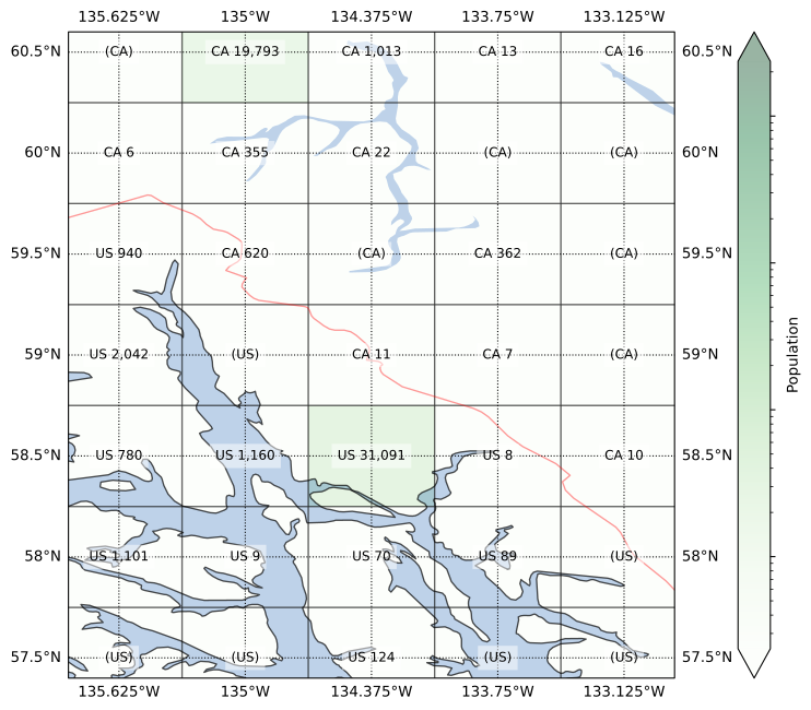
I think this is one the worlds most beautiful places: the water, the forests, the mountains, the wildlife, the snow. It must be an absolutely magical place—at least when the cruise ships are out of reach of your eyes, ears, and nose. As the map shows, not a lot of people live in this region, other than in the capitals Juneau and Whitehorse. One thing might be related to the other.

Despite the low population numbers, this border used to be contentious more than a century ago. Much more recently, there was even a “war” there, albeit “pacific” was part of its name. Although as recently as last week (at the time of writing), a new possible solution to the border issues was diplomatically proposed by a prominent leader involved. In the meanwhile, it wasn’t too hard for me to fill in the missing codes for my grid.

And finally, after so many conflicts and disputes, I figured we should end our tour on a more chill and peaceful note. Last stop, the Southern Levant:

Yeah… It’s hard to come up with anything to say here that doesn’t sound flippant, so I will refrain from doing so.

Conclusions

This exercise was a fun excuse to read up on some interesting places from all over the world. I don’t think there’s a lesson to be learned here other than maps are cool.

August 20, 2026

Countdown to Tram 19

Pre-intro post scriptum

Oh the irony… This was the original post when I had the idea of making this blog. It centered around me complaining about how things always get delayed, starring Delft’s tram line 19 as the example of how something seemingly so simple ends up being late by several years.

I compiled the data at the end of 2024, made the plot in January 2025, and half-wrote the post in April 2025. I then got busy due to a case of increase in scope of my nuclear family, and the website was sent back to the dusty unrealized personal projects shelf.

I have made the commitment of only making this whole blog live once I had made at least 5 posts (check) and had finished this one, The Original Post. So here it goes. I only updated the plot because I found a new data point to add to it.

Long winding intro

When I’m feeling discouraged about the present, I like to think of nice things I can look forward to. These include, of course, major construction projects promising to make life better when completed. New transit infrastructure, for example.

But if you have ever followed such a project, you probably already realize how this coping mechanism is certain to backfire. Accepting the inevitability of multiple delays and cost overruns reveals that checking in on these projects is only yet another thing to feel angry about.

They say acceptance is the last stage of grief, and since I’m here to procrastinate, that will have to wait. Line 19 of the Haagse Tram is as good as any candidate for official hopium supplier to my ADHD-saddled brain. A new tram line extension that would pass right by my workplace at the Delft University of Technology, connecting it to the city’s center and its railway station. It is not just a good bit of infrastructure, but one that would benefit me directly.

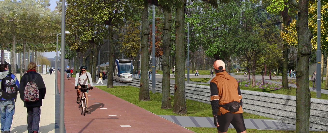
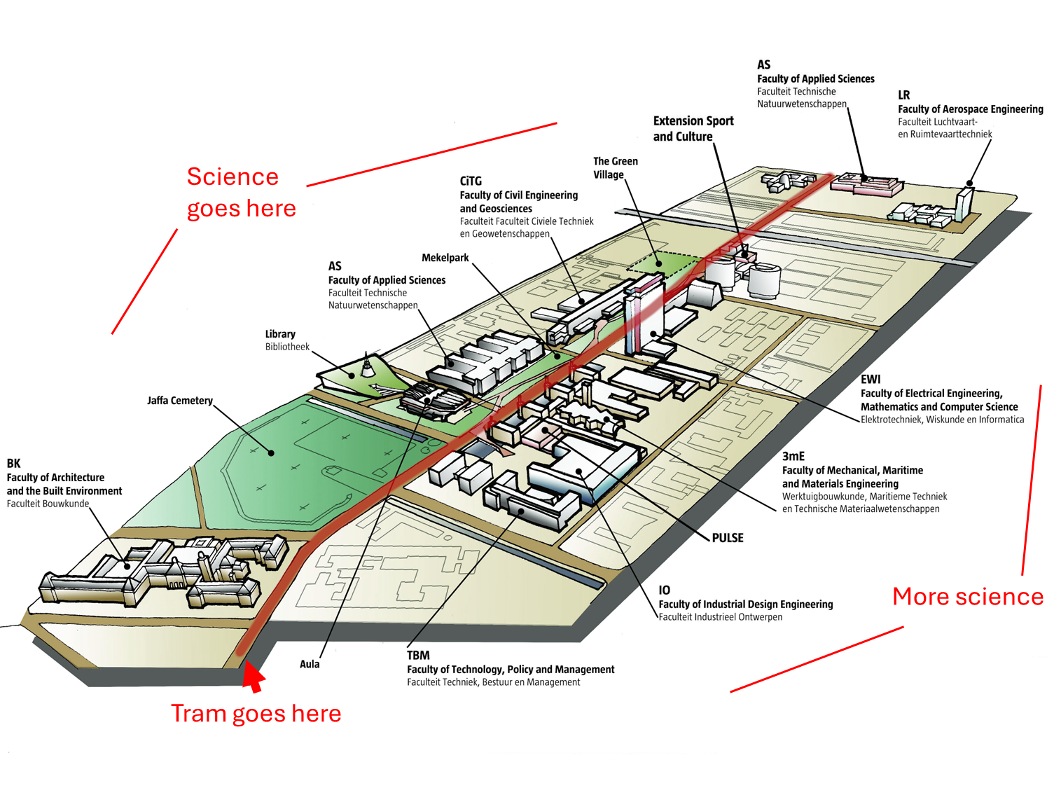
The line is impossible to miss. It cuts through the campus right down the middle, flanked on both sides by the various buildings sheltering the great minds that… apparently were against the line being positioned there? Just think of the impact on the poor parking facilities, or the harm it would do to the concept of the campus! We should be scared that one day the line could potentially be upgraded to an even scarier form of transport, light rail (sneltram is the term used)!

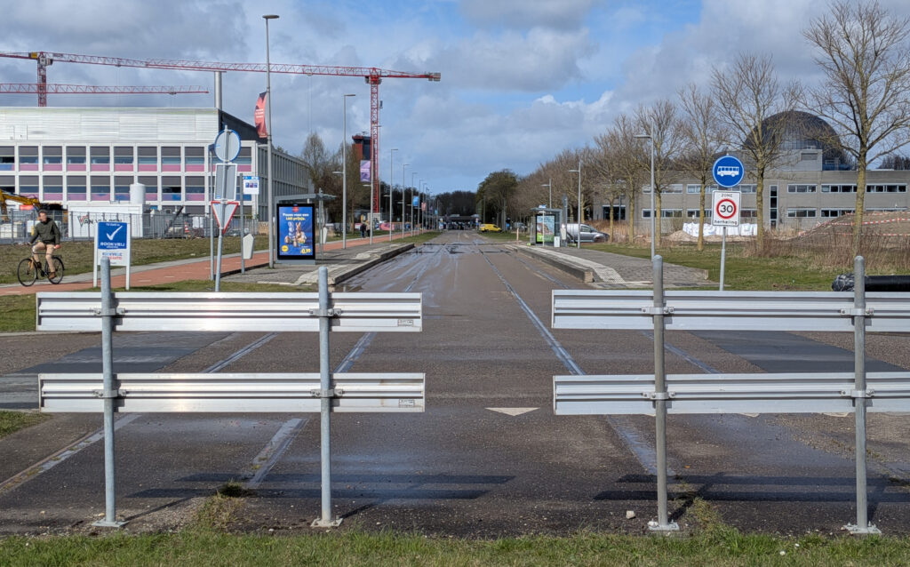
I presume that the municipality won against the visionaries at the Executive Board of TU Delft, because whenever you had to go from one building to another, there it was, at the very center of it all. Those unmistakable trails of extruded steel buried flush with the concrete pavement, on which buses ride with frequency, collecting students and the occasional confused visitor, unsure why there are no trams to be seen on top of the suspiciously rust-tinged rails.

In anticipation for the trams, tracks were installed sometime before I joined the university in 2019. Since then, opening day has always been just around the corner—like the bus that should have arrived three minutes ago according to the timetable, which any moment now should get unstuck from traffic and come to your rescue. But the ride never ends, because as of early 2026 tram 19 is yet to even start riding through TU Delft.

This feels unjust. It feels like I am constantly being cheated out of the final gratification of this obsession. If there is no ultimate benefit, have I just been wasting my time dwelling in anticipation? It feels like the world is rigged such that good things never actually happen. It makes me want to look at the project closer so that either I find the hope and positivity I was looking for in the first place, or at least I find definitive proof that this is really unfair—that things are just systematically hopeless, and I am the clueless sucker who keeps pulling the lever on the slot machine expecting a good outcome.

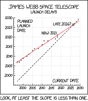
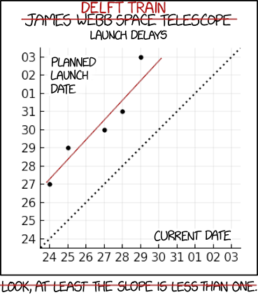
Thankfully, there is always a relevant xkcd. Long before I knew about public transit in these lowlands, I looked forward to the greatest space observatory ever, the James Webb Space Telescope. Same deal: cool nerdy contraption promised to be delivered in the future. Sadly, the project was also infamous for multibillionairily large delays. That comic from 2018, 15 years after the signing of the construction contract and 3 years before the eventual launch of the telescope, managed to tell that story in a way I did not think was possible.

The graph remarkably captured that feeling I had; it contained the proof that we were being constantly let down. Not being as negative as I am, however, the comic has a positive hopeful message, that at least the slope is less than one. To optimism’s credit, the spacecraft did launch eventually—in fact, it did so at the end of 2021, just as the last (non-projected) point suggested.

So that’s the prompt: I wanted to apply the same analysis to other such projects. That is, make the same plot for other cases, exposing the ugly truth about delays that every press release and ribbon cutting ceremony erase with determination. The idea stuck with me, and eventually I saw Tram 19 as a good subject to try this with.

First trial (of the plot, not the tram)

Sorry, one more stop on our way. This is a tale of belatedness after all. In truth, the first opportunity to try out this plot format actually came from another bit of transit infrastructure.

As part of a wider program to increase train frequencies in the southern part of the Oude Lijn, which connects the second and third largest metro areas of the Netherlands, a decent portion of this right of way was being upgraded from 2 to 4 tracks. This included reactivating two platforms at the Schiedam Centrum station which used to go to the sea at Hoek van Holland, as well as reconnecting them to the tracks towards Delft and rearranging the track layout accordingly. The result would be more Sprinter trains (that’s the local service), six per hour at peak instead of four, and capacity for extra Intercity trains (the longer distance service) that wouldn’t necessarily stop at Schiedam.

That would be great for me. 15-min intervals are not bad at all, although by that time the timetable annoyingly had a Sprinter in alternating intervals of 10 and 20 minutes. But 10-min is the magical threshold when I wouldn’t even bother looking at the clock before leaving for the station. No more rushing or detouring for a frikandelbroodje when the next train didn’t align with my morning RNG seed.

But as the saying goes, no geen-trein, no gain. Or something like that.

The Dutch seem to love to renovate things. I guess that’s the unadvertised price of having well-maintained infrastructure: maintenance is annoying. Summer vacation is understandably the preferred time for public inconvenience. Quoting myself at the time, complaining to my coworkers:

“To recap: from July 13 I won’t be able to take the footpath I usually take (which will be closed) to get to the train station, where I won’t be able to catch the train I usually get (which will not run) to the other train station, from which I won’t be able to cross the bridge I usually cross (which will be closed) to get to the office. But none of that matters, because I won’t be able to work at the office (which will also be closed). Cool”

Replacement bus service would run instead of the train from July 13–27. Brought to you by completely clueless Croatian coach drivers who might have never been to the Netherlands before, only speak Croatian, and whose employer I’m guessing offered the lowest price to NS. It was actually fine; and the drivers too, I was just amused by how lost they were on the first day. Still, the longer, less comfortable journey was extra annoying in the heat of summer. Especially when carrying a toddler along, who is not entitled to her own seat.

A mere two days before the restart of service and a delay of a couple of days was announced. Halfway through the now four-day wait, a new delay: just one more day. At least the slope is less than one.

In an unexpected turn of events, the next two days brought more delays. Plus one, then plus three days. Out of frustration, the following figure was born:

But despite the setbacks, it was all good in the end. In fact, trains even ended up running a day earlier than the last forecast plotted. The reason for the delays was that they couldn’t finish the signaling system in time, and the people who knew how to do that were all busy after the time window originally scheduled for the job: “However, these skilled workers are currently difficult to find. This is due, among other things, to a tight labor market”. I love how, in the best economic system ever devised, low unemployment is a worrisome bad thing labeled as tight labor market.

Back to the tram

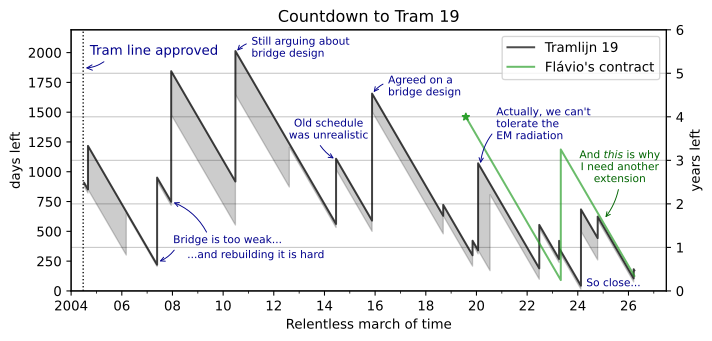
I really liked the format of that xkcd, but it needed a final adjustment. Drawing a 45° line and an almost 45° line doesn’t do justice to the fact that the latter should be at 0°. Doing a little change of variable, or just tilting your head an eighth-turn to the right while keeping the x-axis steady, reveals a nicer format for what I was looking for. The y-axis becomes “time to launch”, which is expected to always go down at a 45° angle until it hits the ground (maybe I should have flipped it, so it went up to the ceiling?). Crucially, any delay is clearly seen as a straight line “jump” that pushes us away from the big moment, kind of like this.

So my plan for the plot was simple: find out how the opening date of the Tram 19 extension to TU Delft changed over time, and make a “countdown” plot. All I needed was to lookup what was the original planned opening date, and what were all the subsequent ones.

But first, we have to ask the question: what is line 19? The one I’m writing about is a line, the newest, on the tram network of The Hague, a city that line runs through only tangentially. Line 19 connects the town of Leidschendam, through the Hague’s district of Leidschenveen-Ypenburg, to the main train station of the city of Delft, some eight kilometers from the center of the Hague. It opened July 1, 2010; and you can read more about its history on Dutch Wikipedia.

But as evidenced by the article from 2004 I referenced in the introduction, the plan was always for the line to diverge from line 1 at the Delft train station, pass through the TU Delft campus, and terminate at the science park just south of it. This last ~3.5 km bit is the “extension” that is yet to materialize.

The earliest expected “opening date” I could find was “end of 2006”; which is more than 19 years ago! To be fair, it is unclear to me if that was supposed to include the tracks to TU Delft, but the next reference I found from less than two months later mention the full line in 2007.

And here’s another issue: if you say your project will take two or three years to execute, and if we assume that there must be limit on shamelessness somewhere, each delay you announce should not be longer than that. From which we can surmise there must have been something like a dozen different delays over all this time.

I tried looking up old news of this project, and succeeded in finding enough (credible?) articles to compile a list with 25 different points in time when the opening date was mentioned. This was not made easier by my beginner level Dutch and how poorly old internet is preserved. I also never bothered to actually go to a library and do my own research in a more formal, proper way. So it’s very likely that I missed some delays or that there are inaccuracies here or there.

Even when an opening date is given, it is actually almost invariably a date-ish, like “mid-2020”. If you say the project will finish “in 2012”, there is zero chance it will finish on Transit Driver Appreciation Day, also known as March 18. The earliest it can be realistically be expected to finish is like by the International Monkey Day (known in some places as December 14). So there was some language parsing for me to do, which is very subjective. Still, I put on my gullible mask and I treated “2012” as a range from 01-01-2012 to 31-12-2012.

Instead of thinking critically about all those 20+ articles I found and crafting a cohesive narrative covering the story behind this never-ending project, I’ll do the engineer thing and just dump a table with the dates I took from them. Please note that while I didn’t go to a physical library, I did use a news archive system from TU Delft, so the early references might be hard to access from the outside. These “VPNwalled” references are listed below the table. Dates are dd-mm-yyyy. “Low” and “High” form a range that is my interpretation of the quoted date when the line would be put in service.

Reference	Opening date	Low	High
23-06-2004^[1]	n/a	n/a	n/a
08-07-2004^[2]	“end of 2006”	01-12-2006	31-12-2006
31-08-2004^[3]	“2007”	01-01-2007	31-12-2007
06-03-2006^[4]	“end of Dec 2007”	16-01-2007	31-12-2007
25-05-2007^[5]	“2012”	01-01-2012	31-12-2012
14-12-2007^[6]	“2012”	01-01-2012	31-12-2012
13-01-2008	“2012”	01-01-2012	31-12-2012
13-03-2009	“2012”	01-01-2012	31-12-2012
04-06-2010^[7]	“2012”	01-01-2012	31-12-2012
27-06-2010	“2015”	01-01-2015	31-12-2015
12-08-2012	“end of 2015”	01-12-2015	31-12-2015
17-06-2014	“Q2 2017”	01-04-2017	30-06-2017
18-11-2015	“before summer 2020”	01-01-2020	31-05-2020
09-09-2018	“mid-2020”	01-06-2020	31-08-2020
26-02-2019^[8]	“mid-2020”	01-06-2020	31-08-2020
06-11-2019^[9]	“end of 2020”	01-12-2020	31-12-2020
25-01-2020^[10]	“after 2020”	01-01-2021	31-12-2022
15-07-2020^[11]	“end of 2022”	01-10-2022	31-12-2022
17-07-2020	“not before Q4 2022”	01-10-2022	31-12-2022
25-06-2022	“end of 2023”	01-12-2023	31-12-2023
10-03-2023	“end of 2023”	01-12-2023	31-12-2023
07-04-2023	“spring 2024”	01-03-2024	31-05-2024
08-04-2023	“end of Q1 2024”	01-03-2024	31-03-2024
16-02-2024	“second half of 2025”	01-06-2025	31-12-2025
14-10-2024	“June 2026”	01-06-2026	30-06-2026
07-03-2026	“early Sep 2026”	01-09-2026	14-09-2026

[1] (June 24, 2004). Gemeente betaalt miljoenen voor tramlijn 19. Haagsche Courant.
[2] (July 8, 2004). LEIDSCHENDAM-VOORBURG – ‘Het Zijdepark is al niet zo groot’. Haagsche Courant.
[3] (August 31, 2004). DELFT – Onderzoek TU naar schade door tramlijn 19. Haagsche Courant.
[4] FLOOR DE BOOYS. (6 March 2006 Monday). Tramlijn 19 komt eraan. AD/Haagsche Courant.
[5] (May 25, 2007 Friday). Aanleg tram 19 jaar vertraagd. De Telegraaf.
[6](14 December 2007 Friday). Jaren vertraging voor tramlijn 19. AD/Haagsche Courant.
[7] (4 juni 2010 vrijdag). Klap op klap voor laatste stuk van nieuwe tramlijn 19. AD/Haagsche Courant.
[8] (26 februari 2019 dinsdag). Miljoenen weg voor ’gedrocht’. De Telegraaf.
[9] (6 november 2019 woensdag). Sebastiaansbrug tweede helft 2020 open. De Telegraaf.
[10] KARL FLIEGER. (25 januari 2020 zaterdag). Straling verstoort komst van tram naar campus. AD/Haagsche Courant.
[11] Carel van der Velden. (15 juli 2020 woensdag). Help, tram heeft twee jaar vertraging! Sint Sebastiaansbrug open, maar lijn 19 niet. AD/Algemeen Dagblad.nl.

The best I can summarize this history of delays is: they realized the bridge leading to TU Delft needed to be reinforced (somehow that accounts for like 14 years of delay), and the other thing is the university was always concerned by vibrations and electromagnetic radiation affecting their sensitive labs, but in addressing those concerns they failed to account for the new model of trams that were to be used.

The oldest of the GTL8 trams still in service, the model used on line 19 when it opened, are now 44 years old. Line 1, which shares tracks with line 19 in Delft, still uses exclusively them. The newer line, however, has already transitioned to the low-floor RegioCitadis, which weighs 59 tons instead of the 38 of the old trams. This required all the tracks in TU-land to be torn out and replaced with a special construction using special concrete, rubber dampers, and a lot of special cables for shorter and better insulated electric loops. You can read a more thorough retelling of the story here (this one is in English, don’t worry).

In addition to the special measures to reduce vibrations and EMR, the very best engineers and scientists in these Low Lands pulled out the big guns, the most powerful tool they had saved for tough unforeseen challenges just like this. In 2020, they just cut the last kilometer or so of the route. The intellectual NIMBYs still got a win after all. The tram won’t go to the science park or even the southern part of TU Delft, where my faculty is located. I say “southern part” because yes, there is a highway that cuts right through the campus, of course there is (a provinciale weg, technically). Tram 19 will now terminate before crossing under that road.

Oh, and for good measure, it was announced in 2023 that: “The tram only runs on working days from 7.00 to 19.00, every fifteen minutes in off-peak hours and in rush hour every ten minutes. The tram does not run faster than 30 km/h on campus and as soon as the tram starts running, bus line 69 is deleted”. I should point out that bendy-bus 69 does run all the way to the “Technopolis” science park, Monday through Friday, from 7:15 to 23:45.

But at last, they are triumphantly sweeping the floor of the recently installed platforms (not the old ones pictured above, those were built for nothing and will never be used). The first test ride scheduled less than two weeks from the date I am writing this. The wait is almost over.

The Plot

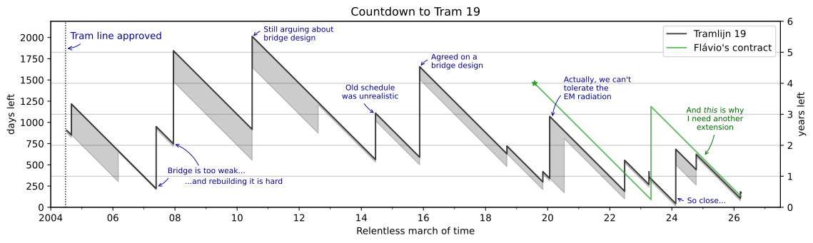
The last ingredient for today’s figure gives it some perspective, and a punchline I suppose. The tram would have been useful for me, if only they hadn’t cut it back and it wasn’t late by so many years. So I decided to make a second line counting down towards the end of my temporary contract. After a three-year extension, I thought I was again on track to use the tram. But further delays mean the opening date is now a month after I leave. Here’s the final figure:

The gray areas represent the “ranges” considered, but the thicker line above is still more prominent. The vertical spikes really serve as a nice visual representation of the “setting back” feeling you get when a new delay is announced. The annotations try to tell the story in a few words, without polluting the figure too much.

Also, those of you who keep a protractor at hand at all times will have noticed that the lines are not actually at 45°. I didn’t use a 1:1 aspect ratio for the axes because this project is so delayed that the figure becomes ungainly. As a bonus, here’s a more chrono-geometrically accurate version:

A final note is that I couldn’t bring myself to project the lines beyond the present day… I tried using the figure to argue why the university should keep me on their payroll, but to no avail. In conclusion, things are always late, but sometimes they eventually arrive. The tram got the last laugh.

March 29, 2026

Overstay in the U-Ess-A
Long winding intro

As an immigrant married to a twice-immigrant, I can’t help but glance at the torrent of ugly immigration related news coming out of the country with the most immigrants in the world (see these fancy plots for the answer). I find it to be a good distraction from all the anti-immigration stuff happening here, where I’ve migrated to.

Fans of the 2017 classic Trump Travel Ban®: Muslim ban? rejoiced when a sequel was released June 2025, dubbed the Second Trump Travel Ban®: Restricting the Entry of Foreign Nationals to Protect the United States from Foreign Terrorists and Other National Security and Public Safety Threats. With a presidential proclamation, the United States imposed a “full” travel ban on 12 countries and a “partial” travel ban on 7 others.

What this meant in practice was the prospective ban on visas being issued to ~~persons~~ foreigners from the targeted countries. “Full” here means a ban on all immigrant and non-immigrant visas. “Partial” means all immigrant plus some major types of non-immigrant visas: B-1/B-2 (business visitor / tourist), F/M (international students), and J (exchange visitor). In both cases, exceptions apply in a number of circumstances, such as for permanent residents, immediate relatives of U.S. citizens, participants of the upcoming FIFA World Cup and Olympic Games, etc. Don’t you love how the Olympics bring people together?

As the American Immigration Council points out in the article linked in the last paragraph, the justification for this was mainly based on three factors. First, the country’s screening and vetting of applicants and information-sharing with the U.S. Second, the likelihood of visa overstay and how easy it is to hand-wave a whole country and say “terrorist”. Third, how cooperative the country is in taking back deportees.

This ban was then expanded on December 2025. As of the start of 2026, nationals of 20 countries are now “fully banned” (including people with a Palestinian Authority travel document), while those of another 20 enjoy a partial ban. This expansion was the expected next step after the government continued its review on the subject, using the same stated rationale.

As this policy memorandum from January 1, 2026 by the U.S. Citizenship and Immigration Services demonstrates, the effect of these proclamations goes beyond stopping the issuing of new visas. Aliens from High-Risk Countries who entered the U.S. on or after January 20, 2021 will have their immigration benefits undergo a comprehensive re-review, requiring a potential interview and re-interview. Also, note that the restrictions are being applied to “aliens with a nationality, country of birth, or aliens who have acquired Citizenship by Investment (CBI) listed in PP 10998”. So just being born in a “high-risk” country is getting you banned, even if you don’t hold that nationality.

Anyways, I am not qualified to do that Family Guy meme to determine how terrorist-harboring each nationality is. So instead, I wanted to look into how U.S. visa overstay rates compare for nationals of various countries. Can these rates really explain the selection of countries for the ban?

An important disclaimer is that I am not looking at the actual merits of these decisions, whether any of this makes sense, or if these developments are good or bad. If you need to be told how to feel about these policies, you should first try soul searching in the lost and found, because you are likely missing something a random blog could not possibly provide. I just wanted to look at some data here, devoid of any deep political discussions.

Keeping up with the news

Things are moving very fast, and between me making the plot and writing this article, a big new restriction was enacted. On January 14, 2026, the U.S. Department of State decided to pause all issuances to immigrant visa applicants who are nationals of 75 countries, effective January 21, 2026. This was done so they could do a “full review of all screening and vetting policies to ensure that immigrants from high-risk countries do not unlawfully utilize welfare in the United States or become a public charge”.

Some of the 39 countries already banned are also included here, plus a fresh new 52. Presumably, divergences in the selections are due to this new restriction being justified more specifically on countries not being trustworthy enough on their own processes and not cooperating enough with the U.S. in sussing out the undesirables. As of February 16, 2026, this pause is still in effect, with no estimate of an end date.

There are cynics who are saying certain religions or ethnicities are being deliberately target with this restriction. Or that personal friendliness or animosity between U.S. and foreign leaders somehow play a role in these decisions. But as I said, these discussions are outside of the scope here. I did redo the plots however, adding a little extra indicator on whether a country is subjected to these newer restrictions or not.

Data

The Department of Homeland Security’s (DHS) Entry/Exit Overstay Report, referenced in the banning proclamations, presents the official fiscal-yearly estimates of how often holders of a non-immigrant visa overstay in the U.S. More precisely, this is how the latest report self-identifies:

This report provides data on expected departures and overstays, by country, for foreign travelers to the United States who were admitted as nonimmigrants at an air or seaport port of entry and were expected to depart in Fiscal Year 2024 (October 1, 2023 – September 30, 2024).

This report is the main evidence cited by that December 2025 proclamation to support the travel bans. So it’s worthwhile to make some notes before going to the figures.

Firstly, technicalities. What is and isn’t in the scope? This is how the report defines “overstay”:

An overstay is defined as a nonimmigrant who was lawfully admitted to the United States but remained in the United States beyond the authorized period of admission. (…) U.S. Customs and Border Protection identifies two types of overstays: 1) individuals for whom no departure was recorded (Suspected In-Country Overstays), and 2) individuals whose departure was recorded after their authorized period of admission expired (Out-of-Country Overstays).

Canada and Mexico are treated differently in the report, as a lot of people from those countries cross into the U.S. somewhere not an “air or seaport port of entry”. Only non-immigrant (which I’m sticking to hyphenate) visas are concerned. Some non-immigrant visas are also out-of-scope: “crewmembers, travelers in transit, and special protected classes under Section 1367”.

Secondly, one should keep in mind that the data come from the United States Customs and Border Protection (CBP) agency of the DHS. So, absent of any ways of independently checking the data, the federal government machine is kind of self-certifying the justifications for its own policies. Which is to say the numbers are only as significant as the credibility of the organization producing them.

Personally, I don’t see any reason why not to trust these specific reports at this point. But it might be worth to understand how the overstay numbers are produced, as they are perhaps overestimates. That American Immigration Council article refers to this piece from 2020, which in turn quotes from a report from a different think tank calling out “flaws” in the CBP/DHS visa overstay reports. The main issue raised is that overstay counts consist of all cases in which a departure could not be verified.

This would also include persons whose visa has expired but are having an application for a different “right to stay” being processed, such as an extension of their visa or a request for asylum. As the Executive Summary of the DHS report puts it:

Determining lawful status requires more than matching entry and exit data. For example, a person may receive a 6-month period of admission upon entry and then subsequently apply for and receive an extension for the period of admission of up to 6 months from U.S. Citizenship and Immigration Services. Identifying extensions, changes, or adjustments of status are necessary steps to determine whether a person has overstayed their authorized period of admission; this report was generated with improvements to data analysis in an automated fashion to better account for these changes.

In total, nearly 46.7 million “in-scope” air or seaport arrivals were expected to depart in FY24. From that, 539 thousand (1.15%) overstays were counted at the end of FY24 (October 1, 2024). Out of those, 483 thousand were suspected in-country overstays (1.04% of total). By February 6, 2025, that number had reduced to 427 thousand (0.92%) due to newly confirmed departures or changes in status.

Visa ABCs

Before getting into the plots, there is a final bit of background information needed. Visas as permissions to enter a country for a specific set of reasons. These can be broadly split into “immigration” and “non-immigration”, depending if the person is moving into the country or just visiting temporarily. As mentioned before, although the bans are (also) completely halting immigration from the affected countries, the overstay report only concerns non-immigration visas.

Within this category of “non-immigration”, there are still several classes of visas. In fact, the overstay report lists 48 different classes within its scope and 27 outside it. The report breaks down overstay counts into three parts, which I am labeling as “B”, “FMJ”, and “Other”:
- B: business or pleasure, consisting of B-1 (business), B-2 (tourism), Waiver-Business, and Waiver-Tourist classes.
- FMJ: students and exchange visitors, consisting of F1/F2 (academic students / their spouse and children), M1/M2 (vocational students / their spouses and children), J1/J2 (exchange visitors / their spouses and children).
- Other: every other in-scope non-immigration visa, including temporary workers and trainees, intracompany transferees, treaty traders and investors, alien fiancées of U.S. citizens and children, Legal Immigration Family Equity LIFE Act, attendants / servants / personal employees of diplomats and other representatives.
The U.S. has a Visa Waiver Program that basically gives the equivalent of a B1/B2 visa access to citizens of certain countries without them having to get a visa first. That’s what they mean when they say, for example, a Dutch person can visit the U.S. without a visa. In practice, you still need an “Electronic System for Travel Authorization (ESTA)”, and not everyone qualifies for this benefit (including if you visited certain countries without the purpose of bombing them). Terms and conditions apply, including a 90-day limit on visits like a B-class visa, so the numbers are presented alongside our “B” category.

For simplicity, because the proclaimed travel bans mention only the “B” and “FMJ” rates as justification, I ignored the “Other” category and looked only at the former two. Remember that these (B, F, M, J) are also the classes of visa being banned under the partial ban.

For the plot, I grouped countries of citizenship into “Full ban”, “Partial ban”, “No ban”, and “Visa waiver”. Separately from the Visa Waiver Program, Canadians can enter the U.S. under most circumstances (and for longer than 90 days). Likewise, citizens from the ~~pseudo-colonies~~ states freely associated with the U.S. have full freedom of movement (terms and conditions apply), i.e. the Marshall Islands, the Federated States of Micronesia, and Palau. For simplicity, I lumped all those four into “Visa waiver”.

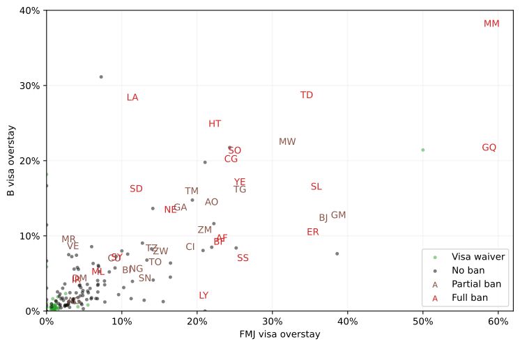
Visas scattered in the wind (it’s just a scatter plot)

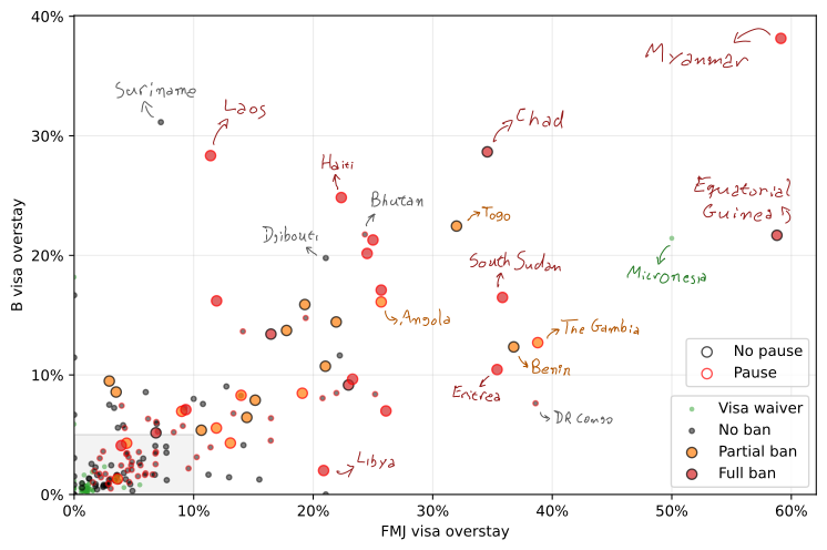
What I did was just take the overstay rates in the FY24 report and make a scatter plot with the “B” rate in the y-axis, and the “FMJ” rate in the x-axis. This choice was based solely on the fact that the latter are usually higher, I wanted the same scale on the axes, and I prefer a wider rather than taller plot (I’m a millennial who views things on a 16:9 monitor).

The main dataviz challenge was on how to indicate what country each point represented. There were 194 nationalities listed after all. An intermediate solution was to replace markers with the two-letter ISO code for the banned countries:

But most people are not going to immediately recognize the codes for these countries. I admit it’s not often I visit a .td, .gm or .bj website. Also, I realized you have to be careful when using letters as markers so that you don’t accidentally form offensive words. Niger to the left of Gabon was enough of a close call.

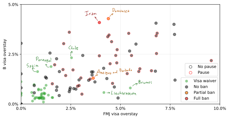
So the final solution was to add annotations to the countries with the highest rates. Because sorting out the layout of this would quickly become too much work if I manually added coordinates for each annotation, I chose instead to do it manually. And by “manually” I mean use my actual hand with a digital pen to write the annotations. Since I’m not used to use a digital pen like this, my setup was probably not ideal, and it took a while to get a passable handwriting.

Anyways, here’s the final figure:

U.S. Visa overstay rate in FY24 per country of citizenship. Decorations refer to visa issuance restrictions as of February 2026. Highlighted region of lowest rates is expanded on the companion figure.

The “Pause” / “No pause” indicators relate to the pause in granting immigration visas started on January 21, 2026. Since its not directly related to the non-immigration visa overstay rates, and they were final additions to the figures (after I had selected the points to annotate), I won’t discuss them further.

So, generally speaking, yes, banned countries tend to have high visa overstay rates. You still have banned nationalities with lower rates than non-banned ones. This could be partially explained by FY23 rates, which can differ a bit from the FY24 values plotted, being used as justifications in the first proclamation from June 2025.

Another reason is that, as described earlier, overstay rates were only one of three “issues” used as justification. This is clearer when looking at the other extreme of the plot, i.e. the countries with the lowest overstay rates:

U.S. Visa overstay rate in FY24 per country of citizenship, zoomed in to rates up to 5%/10%. Decorations refer to visa issuance restrictions as of February 2026.

The U.S. has long added a big red label of “terrorist” on Iran’s figurative forehead, so no surprise on that red dot. Dominica and Antigua and Barbuda, on the other hand, are being banned due to having “historically had CBI without residency”. CBI meaning citizenship by investment.

Another obvious anomaly seems to be Micronesia, the only green dot far out on the plot. No Micronesian needs a U.S. visa under regular circumstances, there is a requirement only if you acquired citizenship by investment or if are naturalized and have not resided there for 5 years yet. The full freedom of movement enjoyed by the members of the Freely Associated States means there should only be an expected departure in these rare exceptions. So the “B” rate is 6 unverified departures out of 28 expected, and the “FMJ” rate is 1 potential overstay from just 2 expected departures. If you look closely at the y-axis of the first figure, you can see also Palau (2/11 and 0/4 for “B” and “FMJ”, respectively) and the Marshall Islands (3/51 B, 0/4 FMJ).

This is an argument raised in the criticism by the American Immigration Council, that the overstay rates “often are based on very small overall numbers of people. For example, the nation of Chad, with a population of over 19 million people, had just 377 suspected B-1/B-2 tourist visa overstays in 2023.” Although I can imagine the counter argument being that “well in that case the ban impacts few people anyway”.

In conclusion, I guess I made a couple of plots with colorful points and text on them. Not sure if that makes up for the feeling of the tightening grip of nationalism and isolationism all around us, while I live in a house with multiple passports, none of which of the country we reside in. People from high-risk countries seem to overstay their visits to low-risk (?) countries, but I’m not sure if we got cause and effect order right between high-risk and high overstay rate.

Also, hi to the immigration officer reading this when deciding whether or not I can visit Disneyland. Who am I kidding, it’ll probably be an AI scraping bot that will ingest this and spit out a Songbun rating with a confidence score.
March 29, 2026
Playground quest

Long winding backstory

Mas não, mas não
O sonho é meu e eu sonho que
Deve ter alamedas verdes
A cidade dos meus amores
E, quem dera, os moradores
E o prefeito e os varredores
Fossem somente crianças
A Cidade Ideal, by Chico Buarque

I grew up in a “metropolitan suburbia”. Which is to say a suburb now solidly nested within one of the world’s largest metropolises. A neighborhood structured as a car-centric suburb, but located in what can only be described as an urban area. I am sure to write more about this in other articles, so I will try to focus here on one aspect of this environment: its child unfriendliness. With my two-week old son sleeping in the next room as I write this, this topic is frequently in my mind these days.

When you are one of the lucky kids that enjoy the modern luxury of freedom from child labor, what do you do with all that time you have? You play, of course. Who doesn’t remember a time when you didn’t want to go to bed because that would mean you’d have to stop playing? Oh, the wonders of childhood… Right, but where do you play?

To middle-class kids in São Paulo, there were several options: at school, inside your own house, inside a friend’s house, in the private playground of your (or your friend’s) condominium, and… that’s kind of it. The obvious omission here being playing on the street.

I am being overly critical, as I certainly played outside countless times, even though my “class” was admittedly above “middle” for our city. Shout out to the playground outside my school, pictured below. But I have always had the sense that kids played less and less outside, specifically in public spaces, with a shift towards the shelter and parental supervision of private spaces.

This actually looks nicer than what I remember from 30 (!) years ago. Source: Google Maps.

It was always clear to everyone that changes in the built environment were related to this. I mean, my granddad used to swim in what later became one of the most polluted rivers in the world. But he was born when the population of the city was – let me check – a twentieth of what it is today. I’m also cheating here, because that was over a century ago, but the point stands. Urbanization then, surely, must be at the root of this trend.

Well, kind of. I would argue that it’s not necessarily that we built the city, but rather how we built it, and for whom.

Car traffic is incompatible with human life, insofar as you tend to die when hit by a moving vehicle. Which is why walking with a toddler is stressful: even when everything is fine, you must maintain unwavering attention to that fragile bumbling newly-biped whose guidance is apparently based exclusively on the principles of Brownian motion. It is a low level of attention that is required, constantly calculating your safety margin if the kid darts straight towards the road and you have to run after them, but it is a level of attention that must be maintained constantly, possibly at the penalty of death. I think that’s why parents feel so relaxed in a shopping mall or a theme park, the calculations of “seconds away from fatal injury” are much more reassuring there.

This is where playgrounds come in. A semi-fenced area where kids can play outside, without as much parental fear of them being run over. Thing is though, most people can’t afford the space and equipment for a worthwhile play area on their own grounds. But perhaps, if we pooled our resources, we could have some sort of big collective “back yard” with recreational equipment made from something other than thin plastic and questionably-welded carbon steel. Public playgrounds also come with the benefit of allowing for socialization, community forming, and up-to-date insight into vandalism in your local area.

I am not really qualified to give an insightful take on this, so instead I’ll just link to two videos from the undisputed world champion in “foreigners glazing up Dutch infrastructure”, Not Just Bikes. This is a good summary of why the Netherlands are a great place to raise children, and this one specifically talks about Dutch public playgrounds.

Short introduction

There seems to be some laws and regulations requiring Dutch municipalities to make sure their public playgrounds are adequately maintained. I’m sure liability concerns are another motivator. From what I understand, this one company sells to municipalities their own information system for conducting inspections and maintenance on these public facilities. But the great thing is they made a website, BuitenSpeelkaart, that shows all public playgrounds from partner municipalities.

I don’t think this tool is very well known, but I found it to be incredibly useful as a parent. In this article, I will go over how I have used it, and write about some of those experiences.

Map of playgrounds

There is a plot I’ve made, but this article is mostly about my appreciation of one that had already existed. In this case, markers on a map showing where all the playgrounds in my city of Schiedam are located.

When you have children, going out to explore the world is very healthy. You might already be tired of “the world”, but young kids still have to give it a try. As an immigrant from a quite different place, I wanted to make sure my daughter got to know the country she was born into, since it feels to me like a privilege we’ve worked for instead of simply being the place where we are. But going out is just as healthy for the parent, as an (often desperate) attempt to not go crazy trying to take care of a child at home.

This is how I found buitenspeelkaart useful. When you are out and about you can check your phone for nearby playgrounds. You can also look up in advance for ideas of new places to explore with your kid. It can show you the way in a city you are visiting, but it also reveals all the spots in your own area that you likely didn’t know existed.

My perception of Dutch city design is that residential areas often have local streets with significant traffic calming, or fully pedestrianized spaces protected by modal filters, that act like public courtyards. If you don’t live there, there is likely no reason to pass by those places, which often feel like communal backyards. It is in those places, sheltered from car traffic, that public playgrounds hide from view. Raising a child gave me this new perspective on the urban environment, and the playground map was a useful tool that guided me in discovering the city I had already been living in for years. There were so many great public places nearby that I had no idea were there!

On the map below of part of Schiedam you can see how tucked away these play areas are, out of the way of through traffic. Also notice just how many of them there are:

See if you can spot the 8 playgrounds here (source: OpenStreetMap). Two more are currently listed on BuitenSpeelkaart: a new one that should be added to OSM, and an older one that has recently been converted into a garden.

As my daughter started walking and making use of playgrounds, I had the idea of printing the map from BuitenSpeelkaart and putting pins on the ones we already visited. It could be a fun quest to explore all of the city’s playgrounds. My rules were that she had to use at least one equipment for it to count, and I would also mark the sport facilities that we happened to walk by, as she was too young to make use of those.

After intense activity during the range of 1–2 years old, our routines changed with more daycare, more toys at home, and a more grown up person with her own say on what we should do. But by that time, having tried out dozens of places, we established our go-tos for different occasions. The big playground in the Princes Beatrixpark is easily the best overall, if you are wondering, but there are a lot of hidden gems. In the end, we were far from 100% completion, but the two sheets of paper remained as a reminder of all the fun we had along the way.

Playgrounds in Schiedam that I visited with my daughter. White and transparent pins are “sport facilities” we just passed by. Other colors have no special meaning.

You will notice that the prints above are slightly different than the current (2026) version of the map. In the last year, Schiedam added a more detailed classification of playgrounds, which differentiate them by size and facilities. Below is an example of the simpler scheme still used in other places.

Simple scheme where red circles are playgrounds and blue ones are places for sport. Source: BuitenSpeelkaart.

The new scheme has more information, although it is a harder to read. As each municipality handles their own facilities, the classification can also be a little inconsistent across borders. That is to say what is considered a “small playground” (kleine speelplek) in one city, might be equivalent to a “neighborhood playground” (buurt speelplek) elsewhere.

Playgrounds in Schiedam, with size classifications. Source: BuitenSpeelkaart.

Quick Dutch recap: speel = play, plek = place, hoekje = (small) corner, kleine = small, buurt = neighborhood, grote = big. For our purposes here, we can ignore the details and just think of four size classes of playground, as exemplified below.

The smallest speelhoekje I have ever encountered. I still appreciate it.

This speelhoekje is quite fancy for its category. But the scale is very deceiving here, this is definitely a (great) spot for a toddler.

This kleine speelplek is about average. Swings, a slide, a spring rocker and some bars: what more could you need?

A buurt speelplek can hit the perfect balance of large size and great equipment while still being quiet.

Grote speelplek is the largest category of playground. They are often found within parks or large green areas.

For today’s figure, my objective was to make my own version of the map for Schiedam, indicating whether or not I have visited each playground. I could have just used photoshop (GIMP) on the screenshot earlier, but this project is all about artisanal, fair trade, data visualization. So I plotted a new map “from scratch”.

(Data) hamster on the playgrounds

The heading is just a shoehorn to mention that data hoarding is called “data hamsteren” in Dutch. There’s so much valuable knowledge that my supervisor and science mentor taught me, and yet this factoid she told us six years ago is what my brain chooses to retain. Anyways, how did I get the playground data?

The buitenspeelkaart website draws the markers on the map locally, which means I could save some .json files from the web browser, in which the playground data was stored. The format was pretty straightforward, giving me a list of locations with their coordinates.

I discarded the purely “sport” locations, and the ones marked as “overig” (other), which I think were all places closed for renovation. With the printed paper full of pins hanging next to me, I manually set each entry as “visited” or not.

Map of the quest

For the base map, I used the default layer of OpenStreetMap, saving rasterized tiles accessed with their API. OSM is not just open, but also much better than Google Maps at showing urban features. This has the benefit of giving my figure a different flavor to buitenspeelkaart, which uses the latter.

For aesthetic reasons, I also wanted to highlight the area of the municipality of Schiedam by partially blanking out everything outside it. So I downloaded the official municipal boundaries, reading them with geopandas.

Thankfully I already knew that the Dutch love to use their own official CRS (coordinate reference system), called Rijksdriehoeksmeting. They’ll have you know that old man Snellius pioneered surveying by triangulation (note that driehoek is Dutch for triangle, or literally “three-corners”). Still, getting cartopy to use the right CRS took me longer than it should have.

Another complication was that I didn’t want to paint the Schiedam shape I just got, but rather the areas outside it. To do that, I made a big Netherlands-sized rectangle and set the Schiedam contour as an interior hole to the polygon (see shapely documentation for more info). But when I plotted this feature, the facecolor was painted everywhere, inside and out. Eventually I figured out what the problem was: the inside of a donut runs counter to the outside—I should have paid more attention to Calculus classes.

Formatting-wise, a major challenge was choosing the right markers. I feel that the buitenspeelkaart icons don’t give a good representation of the significance of each place. If anything, the icon for speelhoekjes, such as that mushroom above, draw more attention than the icon for grote speelpleks. The red and blue colors, while they stand out more from the background, also didn’t seem like the best choice. I thought the map should look like a video game overworld,with the markers indicating whether a “level” was completed or not. In the end, I settled on four different shapes and sizes, with a gold color for “visited” and gray for “not visited”.

There were some other small quirks in preparing the figure too. I used the Century Gothic font instead of the matplotlib default (DejaVu Sans), which didn’t feel “mappy” enough. An unusual arrangement of three legends was chosen as a way of having somewhat tabular counts of playgrounds, and since the shape of the city left plenty of space for them on the sides. Using two different markers for each entry in the legend is also not very conventional, but I think it looks great:

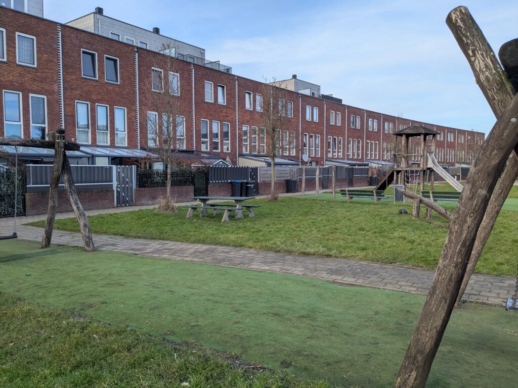
Public playgrounds in the municipality of Schiedam, their size classification, and whether I have visited them with my daughter.

Some 85 years ago the old municipality of Kethel en Spaland was merged into Schiedam. But because they (later) built the A20 highway between them, the city still feels very divided, with the town of Kethel tagging along only for administrative purposes. This is why I thought it best to show the numbers for each part separately.

Quest complete?

Overall, we visited 50 different playgrounds, just in Schiedam—not bad! Some only once, just to be able to put a pin on the map. Others, our favorites, were visited countless times.

Despite this, as the map clearly shows, we were far off from 100% completion. In fact, considering just the “south of A20” area, we got 39% of locations. 46% if we ignore the smallest class, speelhoekjes.

My justification for that is there are just so many playgrounds! To prove my point, I looked up population per age bracket per postal code on CBS. Not that CBS, I mean the Centraal Bureau voor de Statistiek, the Dutch national institute of statistics. There are fewer than 9000 people aged 0–10 years living in Schiedam, giving an average of 59 children per public playground, not counting the speelhoekje variety:

Area Population
0–10 yr Children per playground
(g+b+k) Children per playground
(g+b+k+h)
North of A20 2975 46 36
South of A20 5940 70 53
All of Schiedam 8915 59 46
Ratio of children up to 10 years of age and number of playgrounds excluding and including speelhoekjes.

Perhaps we would build much better cities if we designed them for children instead of cars.

Sour note

Because this post is too rosy for my chronic pessimism, I feel compelled to at least say something bad at the end. Public playgrounds can give you hope in society, but… Maybe some children are just irreparably bad people and we are doomed as a species.

As an example, below are a couple of pictures of (very mildly) defaced playgrounds, with things I futilely wish my children could live their whole lives without ever having to lay their eyes upon. I suppose some people just desperately crave to be noticed, to be seen or heard. But in failing to draw attention for something valuable, I guess being annoying, destructive, or confrontational is a guaranteed way of not feeling insignificant.

[trigger warning: mood ruining edgy offensive messages on playgrounds]

“I am a femboy”

“Adolf Hitler is my sweetie ♡卍”

Trash can (left) and sand on the floor (right). It is an inescapable fact that we all share the same planet as the artists who made these.

So I guess the moral here is that good infrastructure is instrumental in facilitating a healthy, happy and memorable childhood. The public aspect of these installations also help in developing social skills, a sense of shared environment, and a feeling of belonging within society. However, it is still up to the parents to give an education and raise someone into a mature, empathetic, sociable person that isn’t a bratty self-centered hateful dick.

March 29, 2026
The Intercity of the future
Long winding intro

For those who are interested, swaying away to the right there, that’s the Old Bridge, that was replaced by the New Bridge in 1972. Funny thing, the Old Bridge used to be called the New Bridge. Yeah, it’s bit of a funny one
Bus Driver’s Song, by Flight of the Conchords

The Intercity Nieuwe Generatie, ICNG for its closer friends, is the nieuwest train used by the Nederlandse Spoorwegen (NS). But I will have to wait a few decades for the joke above to land, as these trains are meant to replace the locomotive-driven Intercityrijtuig (“Intercity carriages”; ICR), and part of the Intercitymaterieel fleet (“Intercity rolling stock”; ICM). The ICNG joins a further acronym called SNG (Sprinter Nieuwe Generatie), and someday the DDNG (Dubbeldekker Nieuwe Generatie).

The sun has set for the ICR (left), but not yet for the ICM (right).

Some 45 years after the Shinkansen started its operation, the Netherlands opened its own high-speed rail line, named HSL-Zuid. Eventually, a good part of this 300 km/h line between Rotterdam and Amsterdam was downgraded back to low speeds after they realized a series of 10 viaducts were poorly designed. It is currently three years after this discovery, and a month after construction work began on a permanent solution. The current estimate is that repairs will take another 6 years. As this post illustrates, nothing ever goes wrong, so I’m sure the fix will be ready on time.

HSL-Zuid enabled fancy trains to go from the two largest Dutch cities directly to the capitals of Belgium, France, and the UK. But to ~~get back the money they begrudgingly spent~~ to maximize public benefits, the Dutch government also conceded the track to NS for it to run domestic and shorter international services on it. NS International was rearranged, a partnership with KLM was formed, and trains capable of 250 km/h were ordered for a service to Brussels, dubbed Fyra. Delivery of these fast trains was delayed, so NS rented a bunch of TRAXX locomotives from a train landlord (“rolling stock company” if you are feeling charitable) and started the service using the aforementioned ICR carriages.

Long story short, the V250 trainsets started running December 9, 2012, and would have a fondly-remembered career until January 18, 2013. It was decided the best course of action was to rebrand Fyra to Intercity Direct, paint the slow carriages a different color, and forget anything had ever happened.

In 2014, NS said they could tune-up the TRAXX-ICR combo to run at 200 km/h in as little as two and a half years, but it was preferable to buy newer trains instead. This time, they would be less ambitious, with 200 km/h trains to be slotted in between the 300 km/h trains from Thalys / Eurostar. They would buy a model that was already in use elsewhere, and they would test it thoroughly before committing to a start date, which would be no earlier than 2021.

Intercity Defect

A decision was made later in 2014, and in 2016 the ICNG was ordered from Alstom, with entry into service being aimed for 2021 as recently as in 2017. The first unit was received in the Netherlands on May 23, 2020. But, afraid of a second Fyra hitting their proverbial World Trade Center, NS would continue testing for almost three years before there was enough confidence to start passenger service.

Our protagonist, the Intercity Nieuwe Generatie.

The pandemic in 2020 was naturally a good first excuse for the delays. As was a small derailment in Germany, which was not the fault of the two ICNG units being towed, although the optics certainly weren’t ideal for Alstom, who I assume also made the locomotive pulling the consist:

The new trains were a smashing success for Alstom. Photo by F.Thürmer. See video here.

Hopes of a 2022 launch were quashed by discovery of serious technical problems, including poor weld quality and software issues. The news broke only in November of 2022, but the issues had been identified back in March of that year. And in any case, even before that, at the end of 2021, an external report commissioned by the Ministry of Infrastructure and Water Management (I&W) had already established that the original planning was no longer feasible:

Original and 2021 plan. Text translated by me. (source: report from Railistics)

Original and 2021 plan. Original Dutch text. (source: report from Railistics)

But the wait was over when, on April 19, 2023, passengers boarded the ICNG in commercial operation for the first time. After which, the new trains immediately ran into technical issues (the very first day, if you were too lazy to translate the article linked). One day before start of operation, the Secretary of Infrastructure and Water Management sent a letter to the House of Representatives recounting this history of delays and updating them on the current outlook: defective trains would be returned to the factory in Poland for fixes and retrofits, and the last train should roll out of the production line only in 2025. Scheduling risks had been raised earlier in 2023 by a second external review commissioned by the I&W, as promised to the House:

Plan in early 2023: “Planning scenario I is no longer sustainable: the introduction of trains to Amsterdam-Breda is expected to still take place in 2023, between Q2 and Q4, but there will be a delay of at least several months in the introduction of the first trains.” Text translated by me. (source: report from Railistics)

Plan in early 2023: “Planning scenario I is no longer sustainable: the introduction of trains to Amsterdam-Breda is expected to still take place in 2023, between Q2 and Q4, but there will be a delay of at least several months in the introduction of the first trains.” Original Dutch text. (source: report from Railistics)

The narrative that NS put out after launch was that those problems were improving, although half a year later the ICNG’s track record wasn’t really stellar. And as that last article reported, despite all delays up to that point, NS was promising that deliveries would pick up pace and all 99 units would be in operation by early 2026.

Come 2024 and 10 extra units were ordered for international services (I go over the variants below), bringing the total to 109. But delivery of new trains is so slow that Germans start to wonder why there are so many trains parked on their tracks for months now. On July 26, the NRC newspaper publishes this amazing article investigating the whole story, and doing a much better job than I ever could at describing this situation. NS puts out a news brief the same day with their (indirect) response.

So, just a quick list of officially acknowledged technical issues that affected the ICNG:
- Defects in welding the aluminum body, compromising their lifespan.
- Erroneous indications of brake failure.
- Interior sliding doors not working properly.
- Water ingress through the cabin door.
- Noisy and uncomfortable climate control system.
And a list of additional issues mentioned anonymously by a conductor, which are not necessarily systemic:
- Fire door not working.
- Adhesive wrap peeling out.
- Layout of door buttons prone to errors by conductors.
I should also add anecdotal complaints I’ve heard:
- Typically fewer seats than the ICR trains.
- Emergency button placement causes accidental presses too often.
- Significantly less room for trash disposal, causing more littering.
Software updates should be able to fix all of that, especially now with AI and such. So for our plot today I will only look at how delivery went, as it’s already 2026. Wait, I mean how delivery is going.

NS had received enough trains to finally retire the old ICR trains in October 2025, in triumphant fashion. But as we will see, deliveries will continue into 2026 (and beyond?). Relatedly, I rode in an ICNG in September last year (2025) and noticed a strong “fresh train” smell. A quick search on my phone indicated that the unit had started service just a week earlier. The door separating the compartments next to me was out of service.

ICNG variants

Before looking at delivery data, here is a quick explanation of the different variants of the ICNG that NS has ordered (also here):
- ICNG-V: domestic trainset with 5 cars.
- ICNG-VIII: domestic transet with 8 cars.
- ICNG-B: 8-car trainset for international services to Belgium.
- ICNG-D: 8-car trainset for international services to Germany.
Implementation started with the domestic services, with Belgium-bound trains following a few months later. After the ICR carriages were retired, the Intercity Direct services to Brussels were no more. As of December 15, 2025, the era of Eurocity and Eurocity Direct began. Eurocity, the service with more stops, is being operated by Belgium’s NMBS/SNCB, while Eurocity Direct is operated by NS using exclusively the ICNG.

As of writing this, the German-speaking trainsets are still in early testing. They will be used for a new, not yet publicly disclosed international service (extending the The Hague – Eindhoven line to Aachen?).

Tracking trains on tracks

When you are on the platform wondering where is the train that was supposed to have shown up already, you check treinposities.nl. This website (and I’m sure there are others like it) uses real time tracking data provided by NS so that you can follow the (damn) train.

That website also maintains a database of rolling stock, including some extra information added by its community. In the overview page for the ICNG, you can see (depending on when you are reading this) that the last position for a lot of units still reads “Wacht op aflevering” (waiting for delivery).

On the details page for specific trainsets (e.g.) there is a table indicating when their status has changed, such as when they are put in service. It seems most of these are filled automatically when the feed data indicates a trainset is running, but there are also data manually added by moderators. It’s not perfect, but that is fine for our purposes here.

Using this as a data source, my goal was to plot how has delivery gone over time, because despite reassurances from NS, it felt like it was slow. I scraped the website on December 20, 2025 to get a list of when each ICNG trainset was put into service.

There were a few cases of trains that started commercial operation and were later sent back to Poland for rework, which seems to be somewhat recorded in the data. My initial analysis just looked at the date when each operational trainset was put into service (for the last time). It was clear this wasn’t ideal because the plot showed no trains in operation on April 2023. I later refined this to account for trainsets being put into and out of service, with the plot then going both up and down.

The plot

All -V and -VIII trainsets should have been in operation “early 2026”. Let’s see how things were going as of the end of 2025:

Final plot: entry into service of the four variants of the ICNG.

Still a long way to go it seems. In terms of number of domestic cars, we were at $(33*5+13*8)/(49*5+27*8)=58\%$ . No wonder why you can still see crowded trains with just a single 5-car unit during rush. It’s also no surprise that service in the Breda – Rotterdam – Amsterdam route hasn’t been extended to Leeuwarden, Groningen or Eschede yet, although some trains do run all the way to Lelystad now.

The rollout of the smaller -B fleet seems to have been quicker. I’m guessing these units didn’t suffer as much from the weld issues due to entering production later. And maybe the pending commitment to start the EuroCity product with NMBS/SNCB in the 2026 timetable caused the delivery of the -B trains to be prioritized?

Finally, a sequence of work-in-progress plots is show below. These use the first version of data processing, which didn’t account for trainsets being removed from service then being put back into operation.

Work-in-progress: initial plot.

Work-in-progress: formatted plot.

Work-in-progress: annotations added.

Work-in-progress: included number of units for each type.

As always, progress is slow. Both in railway engineering and in me writing posts. But one day in the future, these intercity trains won’t be new anymore. And I hope to get to be old enough to make an update to this plot in which all the lines reach 100%.
March 29, 2026
U.S. Civics Test

Long winding intro

Unlock life in America

It has never been as appealing to be an American as it is today. I thought of making every word of the previous sentence a different hyperlink that illustrates this, but at this point you don’t need me to prove you this fact. However, being an American is not a right, it’s a privilege. A privilege that is, of course, the ultimate ambition of every single non-American in the world. Either you are an American, or an alien who dreams of being allowed to dream the American Dream.

God has only bestowed a select few with the blessing of being a red-white-ang-blue-blooded natural American, emphasis on the white. But because the Land of the Free is also a land of opportunity, if you are a non-citizen who has an outstanding work ethic, share the same American Values, is law-abiding, is not a threat to national security, has filled out all the forms in a timely manner, and has paid all the applicable fees, you may also be afforded the benefit of being allowed to life in the U.S. Eventually, even, you may even achieve the highest honor envied by billions worldwide, and receive citizenship of the United States of America.

But pump your brakes there kid, your decades-long journey gotta start somewhere. Referring back to the very start of the article, may I suggest the following:

Real, official image from the real, official website of the United States government at trumpcard.gov.

Don’t confuse this with a golden visa (derogatory), the Trump Gold Card is a “visa based upon an individual’s ability to provide a substantial benefit to the United States. (…) nonrefundable, $15,000 DHS processing fee. (…) A $1 million gift upon completion of the individual’s vetting is evidence that the individual will substantially benefit the United States. An individual may also need to pay small, additional fees to the U.S. Department of State depending on his or her circumstances.” Under the hood, what happens is the provision of such fees and gifts may expedite your application for an EB-1 or EB-2 visa. This is the visa for aliens with extraordinary ability. Legal terminology, by the way.

I’m trying, but the AI eagle is in my way.

Since I hold no such high ambitions for myself, I have to cope with my FOMO by just maintaining some curiosity on the whole thing; at a safe distance. And as I was reading up on migration news—on the only news source I will ever need—I came across a picture of the finish line I will never be lucky enough to see for myself: the Naturalization Civics Test. The news was that they were aligning it with Executive Order 14161 but, uninterestingly, the content of the test itself remained unchanged.

Having some previous experience with the equivalent test from a different country, I was curious what it looked like, and what would my chances be of passing it. An USCIS officer orally (ew) asks you questions until it is mathematically clear you are either American (12 correct out of 20), or merely an alien who filed Form N-400 (got 9 wrong before the 20^th question).

The thing is though, these 20 Qs are sampled from a list of 128, which are published along with the exact answers you must give. So it is actually just a performative, ceremonial, memorization test, whose goal I guess is to enhance one’s Americaness to an appropriate level before giving them a passport.

Am I civil enough to be an American?

So, could I pass the exam? Yes, I still have good enough short-term memory. If I can memorize 151 Pokémon for nearly three decades and counting, I could memorize a hundred or so mostly one-word answers for a one-time exam. But I wouldn’t even have to, because the questions are quite easy, as you’ll see.

By the way, while the content of the test is still basically the same, they did replace the useless accompanying textbook for applicants to study for the exam. I don’t know why you would go through the trouble of reading all of that instead of going straight to the list of Q&As, but the “A More Perfect Union: Guide to the Monuments and Memorials on the National Mall for the 2008 Civics Test” was a cute harmless way of teaching civics and American history. This had already been replaced (in 2024?) by “One Nation, One People: The USCIS Civics Test Textbook”. Now they did a very minor update to that. For example, see if you can guess which is the 2025 version:

Yes, the new text layer uses a different font, but the old text had already been converted to paths, so who would know (or care) what the exact font was.

I have a theory that everyone thinks they are special. My country is not like other girls, and things of this nature. And because everyone thinks that, they aren’t; we’re all the same. Now, questioning American exceptionalism in these circumstances would surely disqualify you from naturalization and put you on an expedited path to learn about the Second Amendment. But when I took a look at the test questions, I couldn’t help but notice that some of them are not really unique or specific to the U.S. So this got me wondering, just how many questions of the exam could be answered correctly even if you knew absolutely nothing about the U.S?

I set about “taking the test”. Exactly how many questions of the 128 would I get right if I replaced “United States” with “Brazil” (and related wording), and answered accordingly? Then, what exactly would be the odds of passing the test for this unrealistically un-American applicant?

The experiment was fascinating, as some answers matched because the countries are similar, and others matched kind of by coincidence. The exact result depends a bit on how flexible I am in the “translation”. For instance, there were two questions that I was unsure, so I gave myself half a point each:

Two out of the set of 128 questions in the Test.

You could argue that the Declaration of Independence did not say Brazil was free from British control. And no, the Brazilian flag does not have 50 stars.

Tallying up the scores, I counted 55 correct answers. This implies that I am, legally, 43% American. Which, given my parents, actually makes some sense. Another valid interpretation is that Brazil is 43% the same as the U.S., and that the flag below shall be henceforth flown from all staffs in Brasília. Since it used to be the flag of the United States in 1819, this also means Brazil is some 206 years behind. Which, likewise, fair enough.

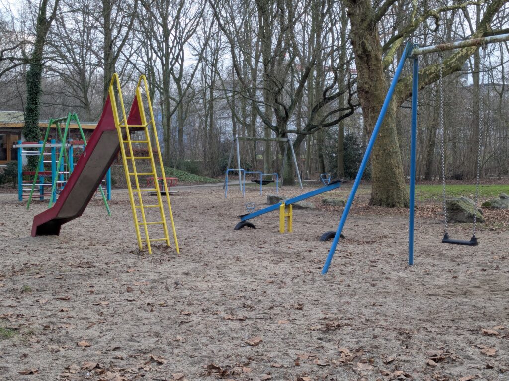
According to the 2025 Naturalization Civics Test, Brazil has an American level of 43%, which grants it 21 full stars.

Fun fact, when Brazil became a republic in 1889, the first idea for a flag was to just copy the American one. Coincidentally, that flag also had 21 stars; the American one had 38 by that time. The following design was used for less than a week before they invented having shame, and a more original design was chosen

This looks ugly, sorry Piauí.

But hold on a minute. An alien needs a score of 60% to pass the exam, so does this mean I’ve failed? Not quite. All is fair through the magic of probabilities. Dusting up some of that knowledge I didn’t pay to learn at college (or was this in high school?), I recall (Wikipedia recalled) that the chances of getting at least 12 passable questions would be:

$\sum_{s=12}^{20} \frac{\binom{55}{s}\binom{128-55}{20-s}}{\binom{128}{20}} = \sum_{s=12}^{20} \frac{\frac{s!(55-s)!}{55!}\frac{(20-s)!(53-s)!}{73!}}{\frac{20!108!}{128!}} = 7.7\%$

So Brazil has a 1-in-(a lucky)-13 chance of a pass. Note that I assumed questions would be picked randomly. I would imagine they actually pick a few questions from each subject, but for the lack of better information, this will do for the analysis. Our plot for today is how the odds change if fewer or more questions match. You’ll find that below.

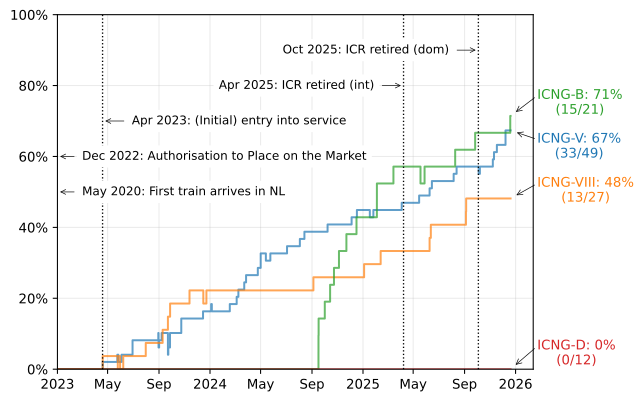
1 in 13 is not great, not terrible. But since naturalization is a serious endeavor, you don’t want to leave it to chance. Therefore, we should psychologically and financially prepare ourselves to take the exam enough times to be confident in a positive outcome. Scientists like to use 95% for some reason, so let’s stick to that:

$1-(1-0.077)^n\ge0.95$

Which gives… $n\ge{}38$ . I don’t know how long it takes for the whole scheduling procedure and so on, but I’m sure it’s all very reasonable. Money-wise, the form to apply for naturalization generally costs $760, or just $710 for an online application. However, you may notice that, as of Q3-2025, the average monthly income in Brazil is R$3,528, which Google tells me is around 630 USD at the moment. This should comfortably put you below 400% of the Department of Health and Human Services Poverty Guideline, which in 2025 sits at an annual income of $62,600 for a 1-person household, meaning you can apply for 50% off discount on the N-400 fee. Hell, the Belastingdiesnt can confirm I still to this day qualify for this generous offer. All told, setting aside $14,440 should be good enough for our exam expenses.

Person, woman, man, camera, TV: 65/20 rule

Because the Test is actually a ceremonial affair that relies just on the sharpness of your memory, there is a small problem. Memory degrades, as the 15 minutes my SDD sometimes takes to boot up demonstrates. So there is a Special Consideration for applicants 65+ years old and who have been lawful permanent residents of the U.S. for 20+ years. In this case, you need just 6 correct answers to 10 questions from a reduced 20-question pool.

This is short enough that I can copy here all the Brazilian answers to give you a taste of the exam. It also makes it reasonable for me to try to verify if the Netherlands would do any better in this regard.

[SPOILER: 20 questions]

Brazil does about the same in the shorter test: 8 out of 20 (40%). But for inexplicable reasons (math), the odds of passing the exam are a little bit better: 8.5%.

The Netherlands does worse, getting only 4 answers correctly, making it impossible to pass. The differences are: Brazil has a president elected every 4 years, who vetoes bills; Native Americans lived there before Europeans; and we have national holidays for Independence Day and Labor Day.

That last one is about names of holidays, not dates. The day Brazilian Will Smith nukes a bunch of aliens (not those aliens!) is September 7. And the Dutch are very American in that they eschew May Day, because communism. In my house, Loyalty Day is the most important day of the year. But the Dutch do go overboard on capitalism, as we have no labor day at all here:

Some people, not me, would even suggest overthrowing a monarchy to fix any eventual clash of days. (source)

Brazil is more American than the Netherlands, okay, but can we do better than that? We have to look in the Americas to get the Native Americans question right. Three of the twenty questions are about specific persons, so it’s impossible to get those. Only the U.S. has a national flag with 13 stripes. Maybe there is another declaration of independence written by a “Jefferson”, but it’s unlikely. No major event happened on 9/11, 2001 in other countries.

There are two other American countries with a “pledge of allegiance” wiki page. But the Bahamas does not have a president. Mexico does, but the president has a 6-year term and might not be able to veto bills (?).

Though unlikely, some other constitution might have 27 amendments, but I’m not going to check that. I think the best hope lies in having a name match. I am not sure how to evaluate the “who is the governor of your state”, because what would I compare it against? Finally, given current answers, I could not find any matches for President, Vice-President, or Speaker of the House. Even with the name “Johnson”. But this could change in the future. We will keep a close eye on this. For the time being, I’m afraid you cannot find a more Americanable country than Brazil.

Plot

I started with a simple plot to see how the odds of passing the test would change with the numbers of answers that matched. In trying to make it prettier, I thought it would be a nice touch to use the colors of the American flag. Which is when an idea came to me and I realized what was the true manifest destiny of the plot: to be in the format of the star-spangled banner.

Because it ended up being quite style-over-function, I still put the finishing touches on a more conventionally formatted line plot, as a more readable version:

Final plot, simple version.

Below is a bonus preliminary version, when I colored the gridlines red. It was at this moment I decided to go all-in on the flag theme. Comparing it to the other two versions shows my line of thought and how the stylistic choices came to be.

Early version of the plot, with gridlines at 10% intervals and 129 star-shaped markers.

Gridlines became the 13 stripes. That spacing is nice because it marks the odds in steps of 1:6, like the common die. After markers became stars, it was clear I should keep only 50 of them. You can notice that their horizontal spacing is not uniform, with a star every 3 questions in the edges and every 2 in the region around the line’s highest inclination (50% odds are between 73 and 74 questions). The aspect ratio also changed to approximately match the 1:1.9 of the flag.

Final plot: your odds of passing the 2025 U.S. Civics Test versus how many answers you remember.

P.S.

I wrote this in 2025. Maybe it was all a moot exercise, and all we have to do to become Americans is wait.

March 29, 2026
Latitude line
(not to be confused with a line of latitude)

Long winding intro

You don’t quite appreciate the North Atlantic Current until you realize that New York City is approximately at the same latitude as Madrid. The snowy, cold, northern city of Toronto has the same latitude as the sunny, pleasant, southern ~~tax-haven~~ port city called Monaco. Also, have you noticed that the majority of people in the Global South actually live in the North, in terms of the… globe, you know?

There are countless little unexpected factoids like these. Seattle is more north than Quebec City, and Paris is further north still. Tokyo is closer to the equator than Melbourne. Sapporo, one of the snowiest cities in the world, is also closer to the equator than Christchurch, where it barely snows.

So I thought it would be interesting to make a plot that discards all other dimensions and reduces cities to their latitude. The idea was to make a vertical line and put cities on it according to their latitude. This should be simple enough, and maybe it will highlight some of these interesting comparisons.

Eventually the idea evolved into making the plot as a transit line diagram, with a selection of large cities represented as “stops” on the line, spaced proportionally to their latitude. This presented an elegant solution to the problem of showing cities with similar values: they could be shown as sort of “interchanges” or “station complexes” in the diagram.

In my experience, a diagram of a single transit line becomes hard to parse visually after ~20 stops, which I’m rounding up to 25 (hey, it’s rounder in base 5). We have about 105 degrees to cover from Wellington to Reykjavik, which means a stop every 4 or 5 degrees. Using the standard conversion rate of 1 degree = 1 km, you can even imagine yourself traveling on a train crossing all those cities in a couple of hours. It used to be faster, but they have to do corrective maintenance on the tracks, sorry.

Next, I will describe which cities and which style to use. Then, the final result.

Ranked competitive ekistics

Which cities should I include in the plot? To save me some time and be a little more scientific, I used a preexisting list of Populated Places, from Natural Earth. These data were prepared to be used as features on maps, so they have properties that allow a selection appropriate for different scales. Using the suggested selection of ("SCALERANK" ≤ 1 Or "FEATURECLA" = 'Admin-0 capital' Or "FEATURECLA" = 'Admin-0 capital alt'), gives 243 cities to choose from. I put everything on a spreadsheet and manually selected our “stops”, trying to space them out by around 4–5 degrees. This is what it looked like:

I always start my travel plans with MS Excel™.

Another consideration was that I wanted to have a mix of places from various continents. The plot should be interesting because it puts cities of very different longitudes together one on top of the other. The grouping in my mind was roughly: “Americas”, “Africa / Middle East / Europe”, “Oceania / (Eastern) Asia”, which is apparent from the spreadsheet excerpt above. I tried to limit these “interchange” stops to places within a ~1.0 degree range, which is why I settled for Chengdu instead of Shanghai, for example.

This longitudinal clustering gave me the idea of having the plot be three lines, one for each continental set, and the interconnections would link up these lines. But this would require a lot of extra effort, so eventually I settled for a simple single line representation. Maybe one day I will revisit the idea.

After the shopping for cities was complete, it all lined up surprisingly well. While it’s still a somewhat arbitrary selection, I think my choices are quite defendable. The only really biased choice was to go for my small hometown of São Paulo instead of the wretched hive of scum and villainy that is Rio de Janeiro, for some reason more favored by the “MIN_ZOOM” gods. But São Paulo has a special thing going for it though, latitudinally-wise: the Tropic of Capricorn (currently) passes over it. I remember being on a road trip when I was a kid and my dad jokingly telling us to duck because we would cross the line. It wasn’t necessarily a special moment, but for whatever reason it is a random fragment of memory that I’ve kept.

In the end, I chose 38 cities for 24 stops, 10 of which were “interchanges”. You can see them below. Also, heads up, Suva is the capital of Fiji. Not that I needed to look that up, but I figured maybe you didn’t know that beforehand.

This is not a map of targets to nuke. Warranty is voided if used as such.

How to draw a line

Before I set about making the diagram, I first had to figure out what such a thing actually looks like. We can all image a metro line diagram in our heads, but if you actually put a few of them side by side, you’ll realize there’s quite a range of styles to choose from.

Snippets of transit diagrams from Rotterdam, London, Paris, and New York.

Taking into account the specifics of our line, the easiness of recreating each style, the home bias I have for the Rotterdam Metro, and my personal preferences, I decided on the line’s format. It would basically be an imitation of the Rotterdam Metro, with notches denoting simple stops and white circles/pills with a black edge denoting interchanges. The line should be red because that is the line I take 4+ days a week.

As an extra, I thought of grouping the line into distinct sections by way of indicating the location of the tropics and the equator. The cute solution I found for this was to pretend each group was a transit zone, which could be done following the style of the London Underground’s map.

In recreating these styles, I ended up going down a calligraphic rabbit hole. Long story short, the font for the city names looks similar to what NS uses, while the zone numbers are similar to what is used in the Tube. And by “similar” I mean I might have copied those fonts from their website, or I might have licensed them, who’s to say. Relatedly, if you were looking for a gift for me, this watch is a perfectly acceptable option.

The plot

One thing I quickly realized was that a horizontal line with text at 45° was a more manageable layout. Fitting the text of multiple-city stops was a bit challenging, but in the end I chose to do everything in a single line, without alternating sides, so as to better align with the markers. Below are some alternatives that didn’t quite work as well:

Not quite my preferred layout.

Speaking of markers, I learned how to hand-make them in Matplotlib:
```
import matplotlib.path as mpath
h = 1.0
rect_up = mpath.Path(
    [[-0.5, 0], [0.5, 0], [0.5, h], [-0.5, h], [-0.5, 0]],
    [mpath.Path.MOVETO, mpath.Path.LINETO, mpath.Path.LINETO, mpath.Path.LINETO, mpath.Path.CLOSEPOLY]
)
```
The markers for the big stops are pill-shaped, defined by circles positioned at the latitude of each city in the stop. If the cities had exactly the same latitude, the marker would be a perfect circle. My solution for these variable-length markers was to actually make them as a white line in front of a larger black line, both with rounded caps:
```
for t in stations_m1_multi:
    x1 = df.loc[t[0]]['LATITUDE']
    x2 = df.loc[t[-1]]['LATITUDE']
    ax.plot([x1, x2], [0, 0], c='k', lw=10, solid_capstyle='round', zorder=2)
    ax.plot([x1, x2], [0, 0], c='w', lw=7, solid_capstyle='round', zorder=3)
```
The zones were also artisanally designed by specifying coordinates for the polygons to be filled. They had to go diagonally at first to align with the text, but everything lined up nicely. Sadly, however, I couldn’t find a good solution to indicate that the transit zones represent Southern/Northern temperate/tropical zones. Adding latitude values or labels like “Tropic of Cancer” seemed to take away from the simplicity of the diagram. It didn’t help that there aren’t good abbreviations or symbols for “tropic” and “equator”. So the “1-2-3-4” might be a bit cryptic, but then again, the whole figure only makes sense if you understand its context.

And so at last, the final plot, in all of its glory:

Final plot: a transit line through major world cities, from South to North.

Oh, if only this was an actual train line, my parents would be just three trains away right now… You know, because I guess I didn’t bother putting Rotterdam itself on the line. But they would still need to take the Metro here, since I don’t live near the train station.
March 29, 2026